Tensors are high dimensional generalizations of matrices. In recent years tensor decompositions were used to design learning algorithms for estimating parameters of latent variable models like Hidden Markov Model, Mixture of Gaussians and Latent Dirichlet Allocation (many of these works were considered as examples of “spectral learning”, read on to find out why). In this post I will briefly describe why tensors are useful in these settings.
Using Singular Value Decomposition (SVD), we can write a matrix $M \in \mathbb{R}^{n\times m}$ as the sum of many rank one matrices:
\[M = \sum_{i=1}^r \lambda_i \vec{u}_i \vec{v}_i^\top.\]When the rank $r$ is small, this gives a concise representation for the matrix $M$ (using $(m+n)r$ parameters instead of $mn$). Such decompositions are widely applied in machine learning.
Tensor decomposition is a generalization of low rank matrix decomposition. Although most tensor problems are NP-hard in the worst case, several natural subcases of tensor decomposition can be solved in polynomial time. Later we will see that these subcases are still very powerful in learning latent variable models.
Matrix Decompositions
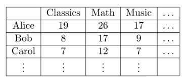
Before talking about tensors, let us first see an example of how matrix factorization can be used to learn latent variable models. In 1904, psychologist Charles Spearman tried to understand whether human intelligence is a composite of different types of measureable intelligence. Let’s describe a highly simplified version of his method, where the hypothesis is that there are exactly two kinds of intelligence: quantitative and verbal. Spearman’s method consisted of making his subjects take several different kinds of tests. Let’s name these tests Classics, Math, Music, etc. The subjects scores can be represented by a matrix $M$, which has one row per student, and one column per test.
The simplified version of Spearman’s hypothesis is that each student has different amounts of quantitative and verbal intelligence, say $x_{quant}$ and $x_{verb}$ respectively. Each test measures a different mix of intelligences, so say it gives a weighting $y_{quant}$ to quantitative and $y_{verb}$ to verbal. Intuitively, a student with higher strength on verbal intelligence should perform better on a test that has a high weight on verbal intelligence. Let’s describe this relationship as a simple bilinear function:
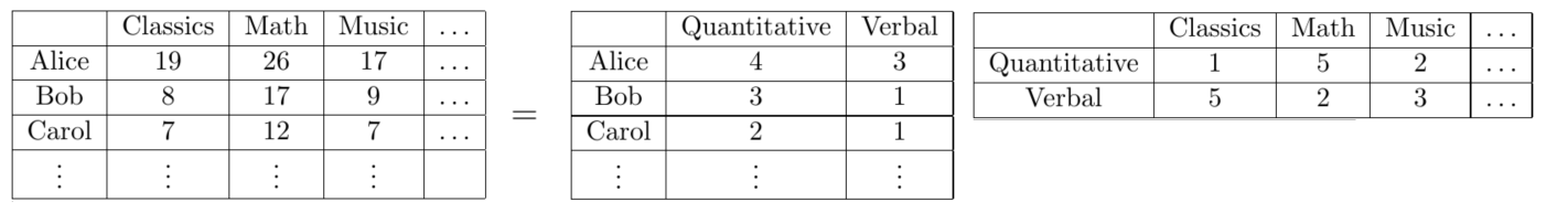
\[score = x_{quant} \times y_{quant} + x_{verb}\times y_{verb}.\]Denoting by $\vec x_{verb}, \vec x_{quant}$ the vectors describing the strengths of the students, and letting $\vec y_{verb}, \vec y_{quant}$ be the vectors that describe the weighting of intelligences in the different tests, we can express matrix $M$ as the sum of two rank 1 matrices (in other words, $M$ has rank at most $2$):
\[M = \vec x_{quant} \vec y_{quant}^\top + \vec x_{verb} \vec y_{verb}^\top.\]Thus verifying that $M$ has rank $2$ (or that it is very close to a rank $2$ matrix) should let us conclude that there are indeed two kinds of intelligence.
Note that this decomposition is not the Singular Value Decomposition (SVD). SVD requires strong orthogonality constraints (which translates to “different intelligences are completely uncorrelated”) that are not plausible in this setting.
The Ambiguity
But ideally one would like to take the above idea further: we would like to assign a definitive quantitative/verbal intelligence score to each student. This seems simple at first sight: just read off the score from the decomposition. For instance, it shows Alice is strongest in quantitative intelligence.
However, this is incorrect, because the decomposition is not unique! The following is another valid decomposition
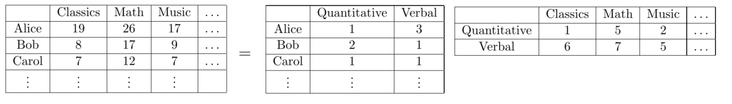
According to this decomposition, Bob is strongest in quantitative intelligence, not Alice. Both decompositions explain the data perfectly and we cannot decide a priori which is correct.
Sometimes we can hope to find the unique solution by imposing additional constraints on the decomposition, such as all matrix entries have to be nonnegative. However even after imposing many natural constraints, in general the issue of multiple decompositions will remain.
Adding the 3rd Dimension
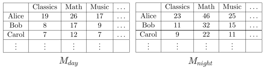
Since our current data has multiple explanatory decompositions, we need more data to learn exactly which explanation is the truth. Assume the strength of the intelligence changes with time: we get better at quantitative tasks at night. Now we can let the (poor) students take the tests twice: once during the day and once at night. The results we get can be represented by two matrices $M_{day}$ and $M_{night}$. But we can also think of this as a three dimensional array of numbers -– a tensor $T$ in $\mathbb{R}^{\sharp students\times \sharp tests\times 2}$. Here the third axis stands for “day” or “night”. We say the two matrices $M_{day}$ and $M_{night}$ are slices of the tensor $T$.
Let $z_{quant}$ and $z_{verb}$ be the relative strength of the two kinds of intelligence at a particular time (day or night), then the new score can be computed by a trilinear function:
\[score = x_{quant} \times y_{quant} \times z_{quant} + x_{verb}\times y_{verb} \times z_{verb}.\]Keep in mind that this is the formula for one entry in the tensor: the score of one student, in one test and at a specific time. Who the student is specifies $x_{quant}$ and $x_{verb}$; what the test is specifies weights $y_{quant}$ and $y_{verb}$; when the test takes place specifies $z_{quant}$ and $z_{verb}$.
Similar to matrices, we can view this as a rank 2 decomposition of the tensor $T$. In particular, if we use $\vec x_{quant}, \vec x_{verb}$ to denote the strengths of students, $\vec y_{quant},\vec y_{verb}$ to denote the weights of the tests and $\vec z_{quant}, \vec z_{verb}$ to denote the variations of strengths in time, then we can write the decomposition as
\[T = \vec x_{quant}\otimes \vec y_{quant}\otimes \vec z_{quant} + \vec x_{verb}\otimes \vec y_{verb}\otimes \vec z_{verb}.\]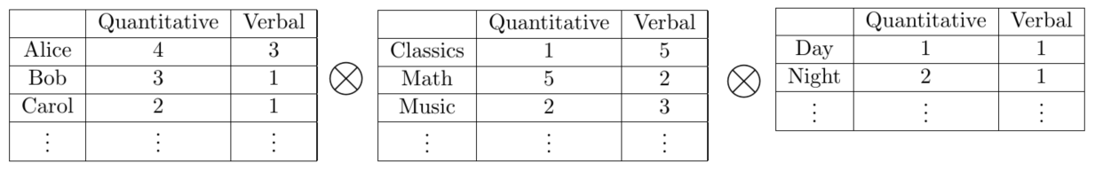
Now we can check that the second matrix decomposition we had is no longer valid: there are no values of $z_{quant}$ and $z_{verb}$ at night that could generate the matrix $M_{night}$. This is not a coincidence. Kruskal 1977 gave sufficient conditions for such decompositions to be unique. When applied to our case it is very simple:
Corollary The decomposition of tensor $T$ is unique (up to scaling and permutation) if none of the vector pairs $(\vec x_{quant}, \vec x_{verb})$, $(\vec y_{quant},\vec y_{verb})$, $(\vec z_{quant},\vec z_{verb})$ are co-linear.
Note that of course the decomposition is not truly unique for two reasons. First, the two tensor factors are symmetric, and we need to decide which factor correspond to quantitative intelligence. Second, we can scale the three components $\vec x_{quant}$ ,$\vec y_{quant}$, $\vec z_{quant}$ simultaneously, as long as the product of the three scales is 1. Intuitively this is like using different units to measure the three components. Kruskal’s result showed that these are the only degrees of freedom in the decomposition, and there cannot be a truly distinct decomposition as in the matrix case.
Finding the Tensor
In the above example we get a low rank tensor $T$ by gathering more data. In many traditional applications the extra data may be unavailable or hard to get. Luckily, many exciting recent developments show that we can uncover these special tensor structures even if the original data is not in a tensor form!
The main idea is to use method of moments (see a nice post by Moritz): estimate lower order correlations of the variables, and hope these lower order correlations have a simple tensor form.
Consider Hidden Markov Model as an example. Hidden Markov Models are widely used in analyzing sequential data like speech or text. Here for concreteness we consider a (simplified) model of natural language texts(which is a basic version of the word embeddings).
In Hidden Markov Model, we observe a sequence of words (a sentence) that is generated by a walk of a hidden Markov Chain: each word has a hidden topic $h$ (a discrete random variable that specifies whether the current word is talking about “sports” or “politics”); the topic for the next word only depends on the topic of the current word. Each topic specifies a distribution over words. Instead of the topic itself, we observe a random word $x$ drawn from this topic distribution (for example, if the topic is “sports”, we will more likely see words like “score”). The dependencies are usually illustrated by the following diagram:
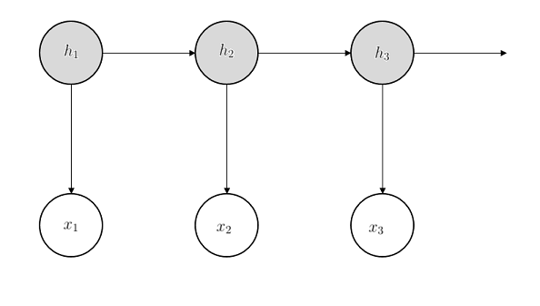
More concretely, to generate a sentence in Hidden Markov Model, we start with some initial topic $h_1$. This topic will evolve as a Markov Chain to generate the topics for future words $h_2, h_3,…,h_t$. We observe words $x_1,…,x_t$ from these topics. In particular, word $x_1$ is drawn according to topic $h_1$, word $x_2$ is drawn according to topic $h_2$ and so on.
Given many sentences that are generated exactly according to this model, how can we construct a tensor? A natural idea is to compute correlations: for every triple of words $(i,j,k)$, we count the number of times that these are the first three words of a sentence. Enumerating over $i,j,k$ gives us a three dimensional array (a tensor) $T$. We can further normalize it by the total number of sentences. After normalization the $(i,j,k)$-th entry of the tensor will be an estimation of the probability that the first three words are $(i,j,k)$. For simplicity assume we have enough samples and the estimation is accurate:
\[T_{i,j,k} = \mbox{Pr}[x_1 = i, x_2=j, x_3=k].\]Why does this tensor have the nice low rank property? The key observation is that if we “fix” (condition on) the topic of the second word $h_2$, it cuts the graph into three parts: one part containing $h_1,x_1$, one part containing $x_2$ and one part containing $h_3,x_3$. These three parts are independent conditioned on $h_2$. In particular, the first three words $x_1,x_2,x_3$ are independent conditioned on the topic of the second word $h_2$. Using this observation we can compute each entry of the tensor as
\[T_{i,j,k} = \sum_{l=1}^n \mbox{Pr}[h_2 = l] \mbox{Pr}[x_1 = i| h_2 = l]\times \mbox{Pr}[x_2 = j| h_2 = l]\times \mbox{Pr}[x_3 = k| h_2 = l].\]Now if we let $\vec x_l$ be a vector whose $i$-th entry is the probability of the first word is $i$, given the topic of the second word is $l$; let $\vec y_l$ and $\vec z_l$ be similar for the second and third word. We can then write the entire tensor as
\[T = \sum_{l=1}^n \mbox{Pr}[h_2 = l] \vec x_l \otimes \vec y_l \otimes \vec z_l.\]This is exactly the low rank form we are looking for! Tensor decomposition allows us to uniquely identify these components, and further infer the other probabilities we are interested in. For more details see the paper by Anandkumar et al. 2012 (this paper uses the tensor notations, but the original idea appeared in the paper by Mossel and Roch 2006).
Implementing Tensor Decomposition
Using method of moments, we can discover nice tensor structures from many problems. The uniqueness of tensor decomposition makes these tensors very useful in learning the parameters of the models. But how do we compute the tensor decompositions?
In the worst case we have bad news: most tensor problems are NP-hard. However, in most natural cases, as long as the tensor does not have too many components, and the components are not adversarially chosen, tensor decomposition can be computed in polynomial time! Here we describe the algorithm by Dr. Robert Jenrich (it first appeared in a 1970 working paper by Harshman, the version we present here is a more general version by Leurgans, Ross and Abel 1993).
Jenrich’s Algorithm
Input: tensor $T = \sum_{i=1}^r \lambda_i \vec x_i \otimes \vec y_i \otimes \vec z_i$.
- Pick two random vectors $\vec u, \vec v$.
- Compute $T_\vec u = \sum_{i=1}^n u_i T[:,:,i] = \sum_{i=1}^r \lambda_i (\vec u^\top \vec z_i) \vec x_i \vec y_i^\top$.
- Compute $T_\vec v = \sum_{i=1}^n v_i T[:,:,i] = \sum_{i=1}^r \lambda_i (\vec v^\top \vec z_i) \vec x_i \vec y_i^\top$.
- $\vec x_i$’s are eigenvectors of $T_\vec u (T_\vec v)^{+}$, $\vec y_i$’s are eigenvectors of $T_\vec v (T_\vec u)^{+}$.
In the algorithm, “$^+$” denotes pseudo-inverse of a matrix (think of it as inverse if this is not familiar).
The algorithm looks at weighted slices of the tensor: a weighted slice is a matrix that is the projection of the tensor along the $z$ direction (similarly if we take a slice of a matrix $M$, it will be a vector that is equal to $M\vec u$). Because of the low rank structure, all the slices must share matrix decompositions with the same components.
The main observation of the algorithm is that although a single matrix can have infinitely many low rank decompositions, two matrices can only have a unique decomposition if we require them to have the same components. In fact, it is highly unlikely for two arbitrary matrices to share decompositions with the same components. In the tensor case, because of the low rank structure we have
\[T_\vec u = XD_\vec u Y^\top; \quad T_\vec v = XD_\vec v Y^\top,\]where $D_\vec u,D_\vec v$ are diagonal matrices. This is called a simultaneous diagonalization for $T_\vec u$ and $T_\vec v$. With this structure it is easy to show that $\vec x_i$’s are eigenvectors of $T_\vec u (T_\vec v)^{+} = X D_\vec u D_\vec v^{-1} X^+$. So we can actually compute tensor decompositions using spectral decompositions for matrices.
Many of the earlier works (including Mossel and Roch 2006) that apply tensor decompositions to learning problems have actually independently rediscovered this algorithm, and the word “tensor” never appeared in the papers. In fact, tensor decomposition techniques are traditionally called “spectral learning” since they are seen as derived from SVD. But now we have other methods to do tensor decompositions that have better theoretical guarantees and practical performances. See the survey by Kolda and Bader 2009 for more discussions.
Related Links
For more examples of using tensor decompositions to learn latent variable models, see the paper by Anandkumar et al. 2012. This paper shows that several prior algorithms for learning models such as Hidden Markov Model, Latent Dirichlet Allocation, Mixture of Gaussians and Independent Component Analysis can be interpreted as doing tensor decompositions. The paper also gives a proof that tensor power method is efficient and robust to noise.
Recent research focuses on two problems: how to formulate other learning problems as tensor decompositions, and how to compute tensor decompositions under weaker assumptions. Using tensor decompositions, we can learn more models that include community models, probabilistic Context-Free-Grammars, mixture of general Gaussians and two-layer neural networks. We can also efficiently compute tensor decompositions when the rank of the tensor is much larger than the dimension (see for example the papers by Bhaskara et al. 2014, Goyal et al. 2014, Ge and Ma 2015). There are many other interesting works and open problems, and the list here is by no means complete.