The language of dynamical systems is the preferred choice of scientists to model a wide variety of phenomena in nature. The reason is that, often, it is easy to locally observe or understand what happens to a system in one time-step. Could we then piece this local information together to make deductions about the global behavior of these dynamical systems? The hope is to understand some of nature’s algorithms and, in this quest, unveil new algorithmic techniques. In this first of a series of posts, we give a gentle introduction to dynamical systems and explain what it means to view them from the point of view of optimization.
Dynamical Systems and the Fate of Trajectories
Given a system whose state at time $t$ takes a value $x(t)$ from a domain $\Omega,$ a dynamical system over $\Omega$ is a function $f$ that describes how this state evolves: one can write the update as [ \frac{dx(t)}{dt} = f(x(t)) \ \ \ \mathrm{or} \ \ \ x(t+1)=x(t) + f(x(t))] in continuous or discrete time respectively. In other words, $f$ describes what happens in one unit of time to each point in the domain $\Omega.$ Classically, to study a dynamical system is to study the eventual fate of its trajectories, i.e., the paths traced by successive states of the system starting from a given state. For this question to make sense, $f$ must not take any state out of the domain. However, a priori, there is nothing to say that $x(t)$ remains in $\Omega$ beyond $x(0).$ This is the problem of global existence of trajectories and can sometimes be quite hard to establish. Assuming that the dynamical system at hand has a solution for all times for all starting points, and $\Omega$ is compact, the trajectories either tend to fixed points, limit cycles or end up in chaos.
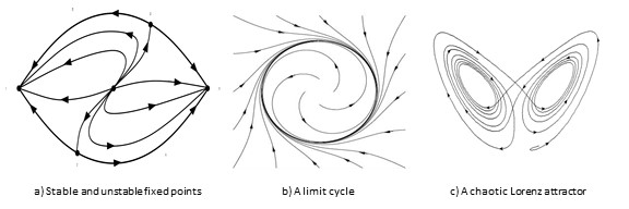
A fixed point of a dynamical system, as the name suggests, is a state $x \in \Omega$ which does not change on the application of $f$, i.e., $f(x)=0.$ A fixed point is said to be stable if trajectories starting at all nearby points eventually converge to it and unstable otherwise. Stability is a property that one might expect to find in nature. Limit cycles are closed trajectories with a similar notion of stability/unstability, while limits of trajectories which are neither fixed points or limit cycles are (loosely) termed as chaos.
What do Dynamical Systems Optimize?
For now, we will consider the class of dynamical systems which only have fixed points, possibly many. In this setting, one can define a function $F$ which maps an $x \in \Omega$ to its limit under the repeated application of $f.$ Note that to make this function well-defined we might have to look at the closure of $\Omega.$ This brings us to the following broad, admittedly not well-defined and widely open question that we would like to study:
Given a dynamical system $(\Omega,f)$, what is $F$?
When $f$ happens to be the negative gradient of a convex function $g$ over some convex domain $\Omega,$ the dynamical system $(\Omega,f)$ is nothing but an implementation of gradient descent to find the minimum of $g$, answering our question perfectly.
However, in many cases, $f$ may not be a gradient system and understanding what $f$ optimizes may be quite difficult. The fact that there may be multiple fixed-points necessarily means that trajectories starting at different points may converge to different points in the domain– giving us a sense of non-convexity. In such cases, answering our question can be a daunting task and, currently, there is no general theory for it. We present two dynamical systems from nature – one easy and one not quite.
Evolution and the Largest Eigenvector
As a simple but important example, consider a population consisting of $n$-types which is subject to the forces of evolution and held at a constant size, say one unit of mass. Thus, if we let $x_i(t)$ denote the fraction of type $i$ at time $t$ in the population, the domain becomes
$\Delta^n=\{x \in \mathbb{R}^n_{>0}: x \geq 0 \; \mathrm{and} \; \; \sum_i x_i=1 \},$ the unit simplex.
The update function is
[ f(x)= Qx - \Vert Qx \Vert_1 \cdot x ]
for a positive matrix $Q \in \mathbb{R}_{>0}^{n \times n}.$
The properties of a natural environment in which the population is evolving can be captured by a matrix $Q,$ see this textbook which is dedicated to the study of such dynamical systems. Mathematically, to start with, note that $f$ maps any point in the simplex to a point in the simplex. Thus, starting at any point in $\Delta^n,$ the trajectory remains in $\Delta^n.$ What are the fixed points of $f$? These are vectors $x \in \Delta^n$ such that $Qx=\Vert Qx \Vert_1 \cdot x$ or the eigenvectors of $Q.$ Since $Q>0,$ the Perron-Frobenius theorem tells us that $Q$ has unique eigenvector $v \in \Delta^n$ and, starting at any $x(0) \in \Delta^n,$ $x(t) \rightarrow v$ as $t \rightarrow \infty.$ Thus, in this case, simple linear algebra can allow us to deduce that $f$ has exactly one fixed point and, thus, we can answer what is $f$ achieving globally: $f$ is nothing but nature’s implementation of the Power Method to compute the maximum eigenvector of $Q$! Biologically, the corresponding eigenvalue can be shown to be the average fitness of the population which is what nature is trying to maximize. It may be worthwhile to note that the maximum eigenvalue problem is non-convex as such.
Solving Linear Programs by Molds?
Let us conclude with an interesting dynamical system inspired by the inner workings of a slime mold; see here for a discussion on how this class of dynamics was discovered. Suppose $A \in \mathbb{R}^{n \times m}$ is a matrix and $b \in \mathbb{R}^n$ is a vector. The domain is the positive orthant $\Omega = \{x \in \mathbb{R}{^m}: x>0 \}.$ For a point $x \in \mathbb{R}^m,$ let $X$ denote the diagonal matrix such that $X_{ii}=x_i.$ The evolution function is then: [ \frac{dx}{dt} = X ( A^\top (AXA^\top)^{-1} b - \vec{1}), ] where $\vec{1}$ is the vector of all ones. Now the problem of existence of a solution is neither trivial nor can be ignored as, for the dynamical system to make sense, $x$ has to be positive. Further, it can be argued in a formal sense that this dynamical system is not a gradient descent. What then can we say about the trajectories of this dynamical system? As it turns out, it can be shown that starting at any $x>0,$ the dynamical system is a gradient descent on a natural Riemannian manifold and converges to a unique point among the solutions to the following linear program, [ \min \; \sum_i x_i \ \ \ \mathrm{s.t.} \ \ \ Ax=b, \ \ x \geq 0, ] which gives us a new algorithm for linear programming. We will explain how in a subsequent post.