This is a followup to an earlier post about word embeddings, which capture the meaning of a word using a low-dimensional vector, and are ubiquitous in natural language processing. I will talk about my joint work with Li, Liang, Ma, Risteski, which tries to mathematically explain their fascinating properties.

We focus on a few questions. (a) What properties of natural languages cause these low-dimensional embeddings to exist? (b) Why do low-dimensional embeddings work better at analogy solving than high dimensional embeddings?

In a future blog post I will address another question answered by our subsequent work: How should a word embedding be interpreted when a word has multiple meanings?

Why do low-dimensional embeddings capture huge statistical information?

Recall that all embedding methods try to leverage word co-occurence statistics. Latent Semantic Indexing does a low-rank approximation to word-word cooccurence probabilities. In the simplest version, if the dictionary has $N$ words (usually $N$ is about $10^5$) then find $v_1, v_2, \ldots, v_N \in \mathbb{R}^{300}$ that minimize the following expression, where $p(w, w’)$ is the empirical probability that words $w, w’$ occur within $5$ words of each other in a text corpus like wikipedia. (Here “$5$” and “$300$” are somewhat arbitrary.)

Of course, one can compute a rank$-300$ SVD for any matrix; the surprise here is that the rank $300$ matrix is actually a reasonable approximation to the $100,000$-dimensional matrix of cooccurences. (Since then, topic models have been developed which imply that the matrix is indeed low rank.) This success motivated many extensions of the above basic idea; see the survey on Vector space models. We’re interested today in methods that perform nonlinear operations on word cooccurence probabilities. The simplest uses the old and popular PMI measure of Church and Hanks, where the probability $p(w,w’)$ in expression (1) is replaced by the following (nonlinear) measure of correlation. (And still the $10^5 \times 10^5$ matrix turns out to have a good low-rank approximation.)

Of course, researchers in applied machine learning take the existence of such low-dimensional approximations for granted, but there appears to be no theory to explain their existence. Theoretical explanations are also lacking for other recent methods such as Google’s word2vec.

Our paper gives an explanation using a new generative model for text, which also gives a clearer insight into the causative relationship between word meanings and the cooccurence probabilities. We think of corpus generation as a dynamic process, where the $t$-th word is produced at step $t$. The model says that the process is driven by the random walk of a discourse vector $c_t \in \Re^d$. It is a unit vector whose direction in space represents what is being talked about. Each word has a (time-invariant) latent vector $v_w \in \Re^d$ that captures its correlations with the discourse vector. We model this bias with a loglinear word production model:

The discourse vector does a slow geometric random walk over the unit sphere in $\Re^d$. Thus $c_{t+1}$ is obtained by a small random displacement from $c_t$. Since expression (2) places much higher probability on words that are clustered around $c_t$, and $c_t$ moves slowly, the model predicts that words occuring at successive time steps will also tend to have vectors that are close together. But this correlation weakens after say, $100$ steps. This model is basically the loglinear topic model of Mnih and Hinton, but with an added dynamic element in the form of a random walk. The model is also related to many existing notions like Kalman filters and linear chain CRFs. Also, as is usual in topic models, it ignores grammatical structure, and treats text in small windows as a bag of words.

Our main contribution is to use the model assumptions to derive closed form expressions for the word-word cooccurence probabilities in terms of the latent variables (i.e., the word vectors). This involves integrating out the random walk $c_t$. For this we need to make a theoretical assumption, which says intuitively that the bulk behavior of the set of all word vectors is similar to what it would be if they were randomly strewn around the conceptual space (this is counterintuitive to my linguistics colleagues because they are used to the existence of fine-grained structure in word meanings).

Isotropy assumption about word vectors: In the bulk, the word vectors behave like random vectors, for example, like $s \cdot u$ where $u$ is a standard Gaussian vector and $s$ is a scalar random variable. In particular, the partition function $Z_c = \sum_w \exp(v_w \cdot c)$ is approximately $Z \pm \epsilon$ for most unit vectors $c$.

We find that in practice the partition function is well-concentrated. After writing our paper we discovered that this phenomenon had been been discovered already in empirical work on self-normalizing language models. (Basic message: Treat the partition function as constant; it doesn’t hurt too much!)

The tight concentration of partition function allows us to compute a multidimensional integral to obtain expressions for word probabilities.

\(\log p(w,w') = \frac{\|v_w + v_{w'}\|_2^2 }{2d}- 2\log Z \pm \epsilon.\) \(\log p(w) = \frac{\|v_w\|_2^2}{2d} - \log Z \pm \epsilon.\) \(PMI(w, w') = \frac{v_w \cdot v_{w'}}{d} \pm 2\epsilon.\)

Thus the model predicts that the PMI matrix introduced earlier is indeed low-dimensional. Furthermore, unlike previous models, low dimension plays a key role in the story: isotropy requires the dimension $d$ to be much smaller than $N$.

A theoretical “explanation” also follows for some other nonlinear models. For instance if we try to do a max-likelihood fit (MLE) to the above expressions, something interesting happens in the calculation: different word pairs need to be weighted differently. Suppose you see that $w, w’$ cooccur $X(w, w’)$ times in the corpus. Then it turns out that your trust in this count as an estimate of the true value of $p(w, w’)$ scales linearly with $X(w, w’)$ itself. In other words the MLE fit to the model is

\(\min_{\{v_{w}\}, C} \quad \sum_{w,w'} X(w,w') \left( \log(X(w,w') - \|v_{w} + v_{w'}\|_2^2 - C \right)^2\) This is very similar to the expression in the GloVE model, but provides some explanation for their mysterious bias and reweighting terms. Empirically we find that this model fits the data quite well: the weighted termwise error (without the square) is about $5$ percent. (The weighted termwise error for the PMI model is much worse, around $17\%$.)

A theoretical explanation can also be given for Google’s word2vec model. Suppose we assume the random walk of the discourse vector is slow enough that $c_t$ is essentially unchanged while producing consecutive strings of $10$ words or more. Then the average of the word vectors for any consecutive $5$ words is a Max a Posteriori (MAP) estimate of the discourse vector $c_t$ that produced them. This leads to the word2vec(CBOW) model, which had hitherto seemed mysterious:

\[\Pr[w|w_1, w_2, \ldots, w_5] \propto \exp(v_w \cdot (\frac{1}{5} \sum_i v_{w_i})),\qquad (2)\]

Why do low dimensional embeddings work better than high-dimensional ones?

A striking finding in empirical work on word embeddings is that there is a sweet spot for the dimensionality of word vectors: neither too small, nor too large. This graph below from the Latent Semantic Analysis paper (1997) shows the performance on word similarity tasks versus dimension, but a similar phenomenon also occurs for analogy solving.

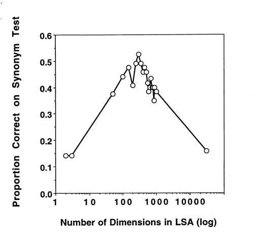
Such a performance curve with a bump at the “sweet spot” is very familiar in empirical work in machine learning and usually explained as follows: too few parameters make the model incapable of fitting to the signal; too many parameters, and it starts overfitting (e.g., fitting to noise instead of the signal). Thus the dimension constraint act as a regularizer for the optimization.

Surprisingly, I have not heard of a good theoretical explanation to back up this intuition. Here are some attempted explanations I heard from colleagues in connection with word embeddings.

Suggestion 1: Johnson-Lindenstrauss Lemma implies some dimension reduction for every set of vectors. This explanation doesn’t cut it because: (a) it only implies dimension $\frac{1}{\epsilon^2}\log N$, which is too high for even moderate $\epsilon$. (b) It predicts that quality of the embedding goes up monotonically as we increase dimension, whereas in practice overfitting is observed.

Suggestion 2: Standard generalization theory (e.g., VC-dimension) predicts overfitting. I don’t see why this applies either, since we are dealing with unsupervised learning (or transfer learning): the training objective doesn’t have anything to do a priori with analogy solving. So there is no reason a model with fewer parameters will do better on analogy solving, just as there’s no reason it does better for some other unrelated task like predicting the weather.

We give some idea why a low-dimensional model may solve analogies better. This is also related to the following phenomenon.

Why do Semantic Relations correspond to Directions?

Remember the striking discovery in the word2vec paper: word analogy tasks can be solved by simple linear algebra. For example, the word analogy question man : woman ::king : ?? can be solved by looking for the word $w$ such that $v_{king} - v_w$ is most similar to $v_{man} - v_{woman}$; in other words, minimizes

This strongly suggests that semantic relations —in the above example, the relation is masculine-feminine—correspond to directions in space. However, this interpretation is challenged by Levy and Goldberg who argue there is no linear algebra magic here, and the expression can be explained simply in terms of traditional connection between word similarity and vector inner product (cosine similarity). See also this related blog post.

We find on the other hand that the RELATIONS = DIRECTIONS phenomenon is demonstrable empirically, and is particularly clear for semantic analogies in the testbed. For each relation $R$ we can find a direction $\mu_R$ such if a word pair $a, b$ satisfy $R$, then

\(v_a - v_b = \alpha_{a, b}\cdot \mu_R + \eta,\) where $\alpha_{a, b}$ is a scalar that’s roughly about $0.6$ times the norm of $v_a - v_b$ and $\eta$ is a noise vector. Empirically, the residuals $\eta$ do look mathematically like random vectors according to various tests.

In particular, this phenomenon allows the analogy solver to be made completely linear algebraic if you have a few examples (say 20) of the same relation. You compute the top singular vector of the matrix of all $v_a -v_b$’s to recover $\mu_R$, and from then on can solve analogies $a: b:: c:??$ by looking for a word $d$ such that $v_c - v_d$ has the highest possible projection on $\mu_R$ (thus ignoring $v_a -v_b$ altogether). In fact, this gives a “cheating” method to solve the analogy test bed with somewhat higher success rates than state of the art. (Message to future designers of analogy testbeds: Don’t include too many examples of the same relationship, otherwise this cheating method can exploit it.) By the way, Lisa Lee did a senior thesis under my supervision that showed empirically that this phenomenon can be used to extend knowledge-bases of facts, e.g., predict new music composers in the corpus given a list of known composers.

Our theoretical results can be used to explain the emergence of RELATIONS=DIRECTIONS phenomenon in the embeddings. Earlier attempts (eg in the GloVE paper) to explain the success of (3) for analogy solving had failed to account for the fact that all models are only approximate fits to the data. For example, the PMI model fits $v_w \cdot v_{w’}$ to $PMI(w, w’)$) but the termwise error for our corpus is $17\%$, and expression (3) contains $6$ inner products! So even though expression (3) is presumably a linear algebraic proxy for some statistical property of the word distributions, the noise/error is large. By contrast, the difference in the value of (3) between the best and second-best solution is small, say $10-15\%$.

So the question is: Why does error in the approximate fit not kill the analogy solving? Our explanation of RELATIONS = DIRECTIONS phenomenon provides an explanation: the low dimension of the vectors has a “purifying” effect that reduces the effect of this fitting error. (See Section 4 in the paper.)The key ingredient of this explanation is, again, the random-like behavior of word embeddings —quantified in terms of singular values— as well as the standard theory of linear regression. I’ll describe the math in a future post.