This post is about my new paper with Rong Ge, Behnam Neyshabur, and Yi Zhang which offers some new perspective into the generalization mystery for deep nets discussed in my earlier post. The new paper introduces an elementary compression-based framework for proving generalization bounds. It shows that deep nets are highly noise stable, and consequently, compressible. The framework also gives easy proofs (sketched below) of some papers that appeared in the past year.
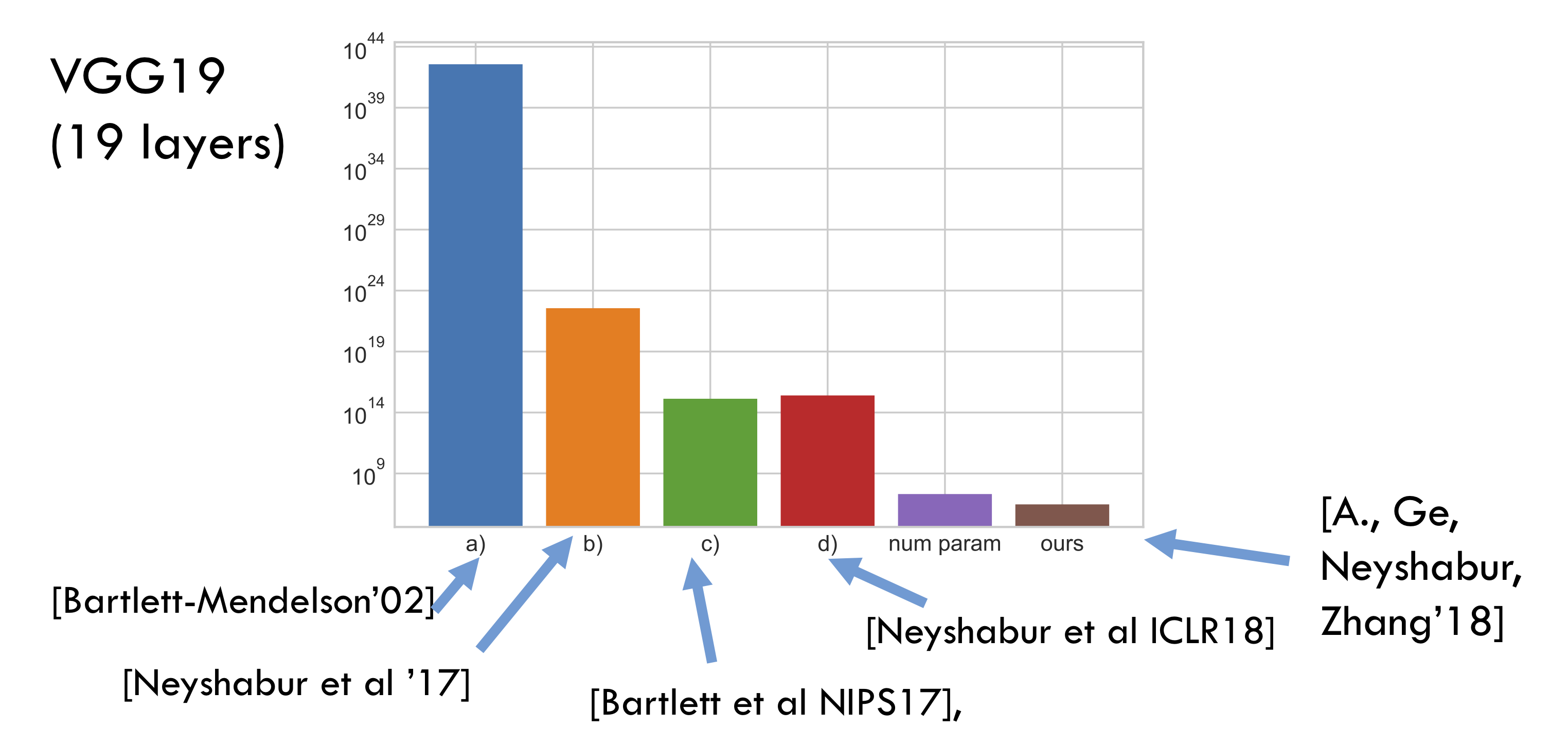
Recall that the basic theorem of generalization theory says something like this: if training set had $m$ samples then the generalization error —defined as the difference between error on training data and test data (aka held out data)— is of the order of $\sqrt{N/m}$. Here $N$ is the number of effective parameters (or complexity measure) of the net; it is at most the actual number of trainable parameters but could be much less. (For ease of exposition this post will ignore nuisance factors like $\log N$ etc. which also appear in the these calculations.) The mystery is that networks with millions of parameters have low generalization error even when $m =50K$ (as in CIFAR10 dataset), which suggests that the number of true parameters is actually much less than $50K$. The papers Bartlett et al. NIPS’17 and Neyshabur et al. ICLR’18 try to quantify the complexity measure using very interesting ideas like Pac-Bayes and Margin (which influenced our paper). But ultimately the quantitative estimates are fairly vacuous —orders of magnitude more than the number of actual parameters. By contrast our new estimates are several orders of magnitude better, and on the verge of being interesting. See the following bar graph on a log scale. (All bounds are listed ignoring “nuisance factors.” Number of trainable parameters is included only to indicate scale.)
The Compression Approach
The compression approach takes a deep net $C$ with $N$ trainable parameters and tries to compress it to another one $\hat{C}$ that has (a) much fewer parameters $\hat{N}$ than $C$ and (b) has roughly the same training error as $C$.
Then the above basic theorem guarantees that so long as the number of training samples exceeds $\hat{N}$, then $\hat{C}$ does generalize well (even if $C$ doesn’t). An extension of this approach says that the same conclusions holds if we let the compression algorithm to depend upon an arbitrarily long random string provided this string is fixed in advance of seeing the training data. We call this compression with respect to fixed string and rely upon it.
Note that the above approach proves good generalization of the compressed $\hat{C}$, not the original $C$. (I suspect the ideas may extend to proving good generalization of the original $C$; the hurdles seem technical rather than inherent.) Something similar was true of earlier approaches using PAC-Bayes bounds, which also prove the generalization of some net related to $C$, not of $C$ itself. (Hence the tongue-in-cheek title of the classic reference Langford-Caruana2002.)
Of course, in practice deep nets are well-known to be compressible using a slew of ideas—by factors of 10x to 100x; see the recent survey. However, usually such compression involves retraining the compressed net. Our paper doesn’t consider retraining the net (since it involves reasoning about the loss landscape) but followup work should look at this.
Flat minima and Noise Stability
Modern generalization results can be seen as proceeding via some formalization of a flat minimum of the loss landscape. This was suggested in 1990s as the source of good generalization Hochreiter and Schmidhuber 1995. Recent empirical work of Keskar et al 2016 on modern deep architectures finds that flatness does correlate with better generalization, though the issue is complicated, as discussed in an upcoming post by Behnam Neyshabur.
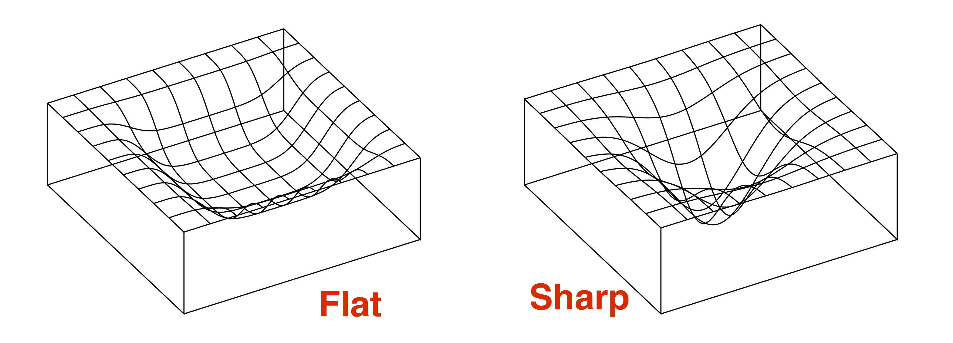
Here’s the intuition why a flat minimum should generalize better, as originally articulated by Hinton and Camp 1993. Crudely speaking, suppose a flat minimum is one that occupies “volume” $\tau$ in the landscape. (The flatter the minimum, the higher $\tau$ is.) Then the number of distinct flat minima in the landscape is at most $S =\text{total volume}/\tau$. Thus one can number the flat minima from $1$ to $S$, implying that a flat minimum can be represented using $\log S$ bits. The above-mentioned basic theorem implies that flat minima generalize if the number of training samples $m$ exceeds $\log S$.
PAC-Bayes approaches try to formalize the above intuition by defining a flat minimum as follows: it is a net $C$ such that adding appropriately-scaled gaussian noise to all its trainable parameters does not greatly affect the training error. This allows quantifying the “volume” above in terms of probability/measure (see my lecture notes or Dziugaite-Roy) and yields some explicit estimates on sample complexity. However, obtaining good quantitative estimates from this calculation has proved difficut, as seen in the bar graph earlier.
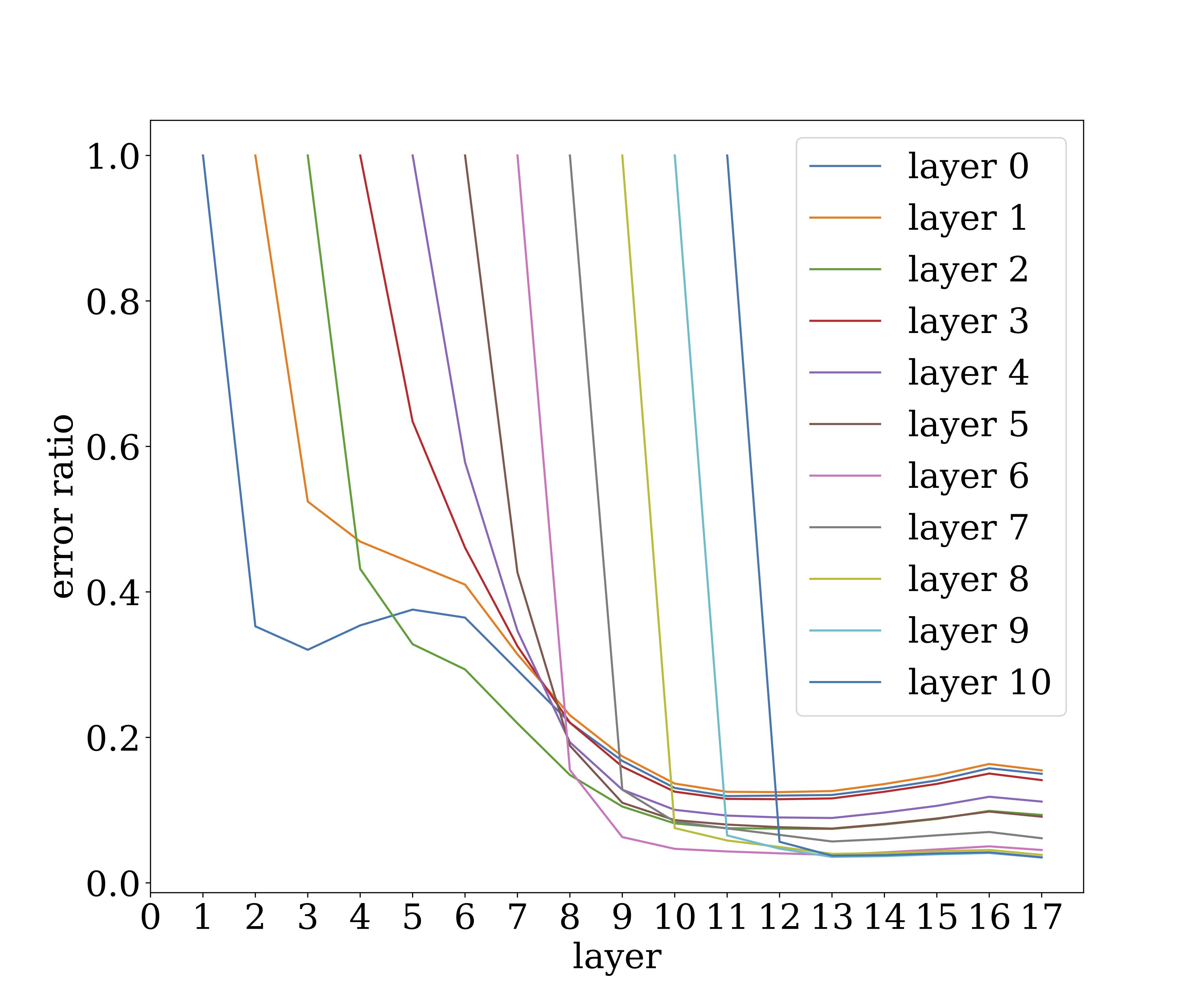
We formalize “flat minimum” using noise stability of a slightly different form. Roughly speaking, it says that if we inject appropriately scaled gaussian noise at the output of some layer, then this noise gets attenuated as it propagates up to higher layers. (Here “top” direction refers to the output of the net.) This is obviously related to notions like dropout, though it arises also in nets that are not trained with dropout. The following figure illustrates how noise injected at a certain layer of VGG19 (trained on CIFAR10) affects the higher layer. The y-axis denote the magnitude of the noise ($\ell_2$ norm) as a multiple of the vector being computed at the layer, and shows how a single noise vector quickly attenuates as it propagates up the layers.
Clearly, computation of the trained net is highly resistant to noise. (This has obvious implications for biological neural nets…) Note that the training involved no explicit injection of noise (eg dropout). Of course, stochastic gradient descent implicitly adds noise to the gradient, and it would be nice to investigate more rigorously if the noise stability arises from this or from some other source.
Noise stability and compressibility of single layer
To understand why noise-stable nets are compressible, let’s first understand noise stability for a single layer in the net, where we ignore the nonlinearity. Then this layer is just a linear transformation, i.e., matrix $M$.
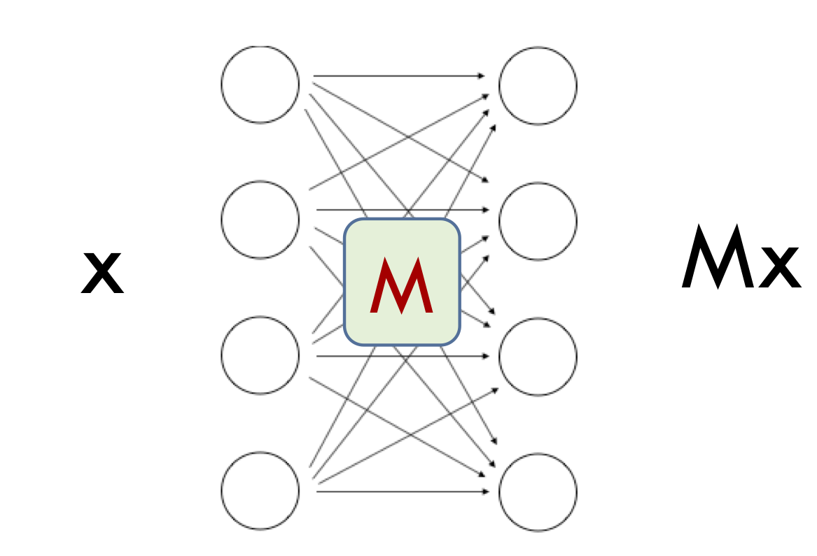
What does it mean that this matrix’s output is stable to noise? Suppose the vector at the previous layer is a unit vector $x$. This is the output of the lower layers on an actual sample, so $x$ can be thought of as the “signal” for the current layer. The matrix converts $x$ into $Mx$. If we inject a noise vector $\eta$ of unit norm at $x$ then the output must become $M(x +\eta)$. We say $M$ is noise stable for input $x$ if such noising affects the output very little, which implies the norm of $Mx$ is much higher than that of $M \eta$. The former is at most $\sigma_{max}(M)$, the largest singular value of $M$. The latter is approximately $(\sum_i \sigma_i(M)^2)^{1/2}/\sqrt{h}$ where $\sigma_i(M)$ is the $i$th singular value of $M$ and $h$ is dimension of $Mx$. The reason is that gaussian noise divides itself evenly across all directions, with variance in each direction $1/h$. We conclude that: \((\sigma_{max}(M))^2 \gg \frac{1}{h} \sum_i (\sigma_i(M)^2),\)
which implies that the matrix has an uneven distribution of singular values. Ratio of left side and right side is called the stable rank and is at most the linear algebraic rank. Furthermore, the above analysis suggests that the “signal” $x$ is correlated with the singular directions corresponding to the higher singular values, which is at the root of the noise stability.
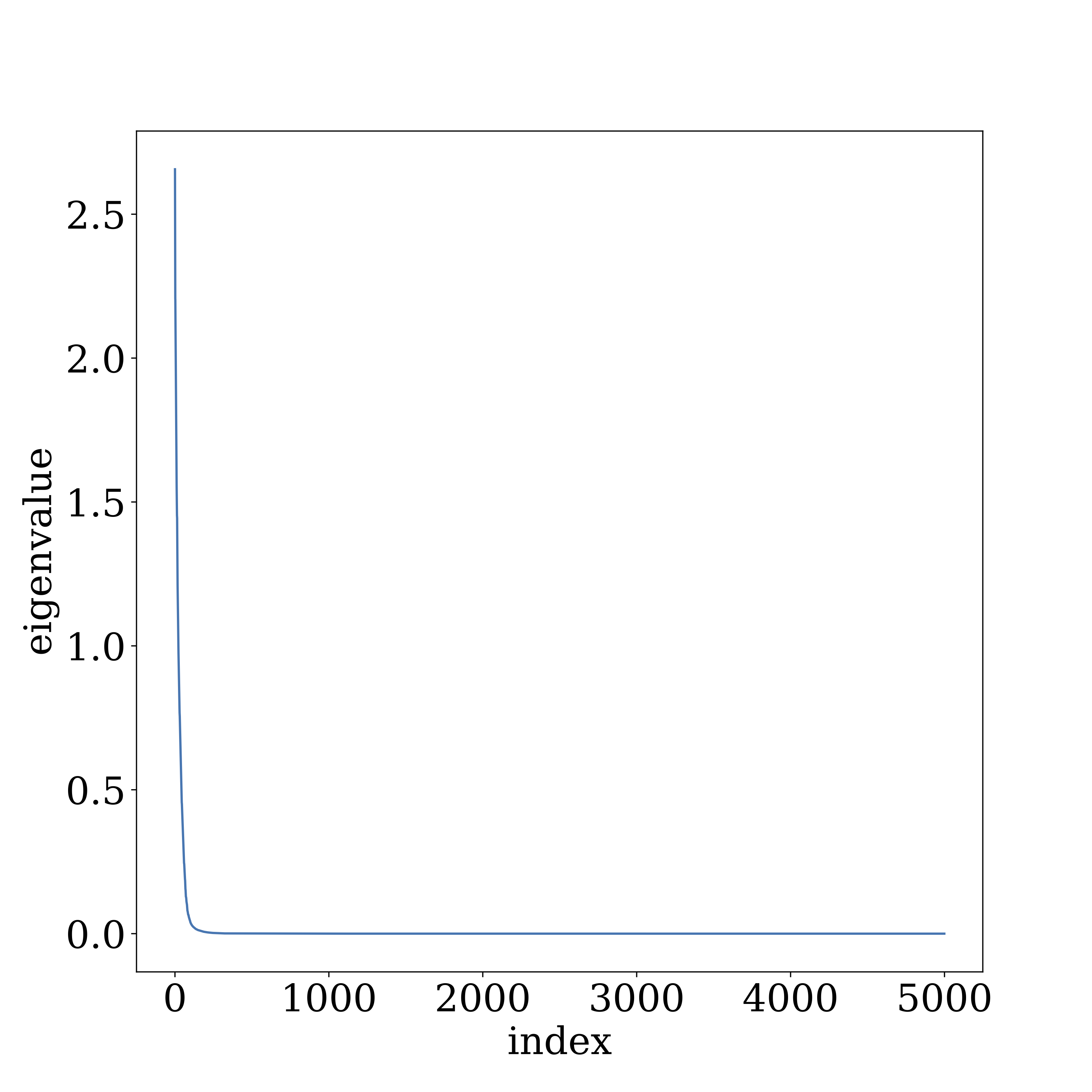
Our experiments on VGG and GoogleNet reveal that the higher layers of deep nets—where most of the net’s parameters reside—do indeed exhibit a highly uneven distribution of singular values, and that the signal aligns more with the higher singular directions. The figure below describes layer 10 in VGG19 trained on CIFAR10.
Compressing multilayer net
The above analysis of noise stability in terms of singular values cannot hold across multiple layers of a deep net, because the mapping becomes nonlinear, thus lacking a notion of singular values. Noise stability is therefore formalized using the Jacobian of this mapping, which is the matrix describing how the output reacts to tiny perturbations of the input. Noise stability says that this nonlinear mapping passes signal (i.e., the vector from previous layers) much more strongly than it does a noise vector.
Our compression algorithm applies a randomized transformation to the matrix of each layer (aside: note the use of randomness, which fits in our “compressing with fixed string” framework) that relies on the low stable rank condition at each layer. This compression introduces error in the layer’s output, but the vector describing this error is “gaussian-like” due to the use of randomness in the compression. Thus this error gets attenuated by higher layers.
Details can be found in the paper. All noise stability properties formalized there are later checked in the experiments section.
Simpler proofs of existing generalization bounds
In the paper we also use our compression framework to give elementary (say, 1-page) proofs of the previous generalization bounds from the past year. For example, the paper of Neyshabur et al. shows the following is an upper bound on the generalization error where $A_i$ is the matrix describing the $i$th layer.
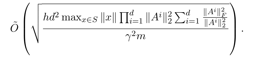
Comparing to the basic theorem, we realize the numerator corresponds to the number of effective parameters. The second part of the expression is the sum of stable ranks of the layer matrices, and is a natural measure of complexity. The first part is product of spectral norms (= top singular value) of the layer matrices, which happens to be an upper bound on the Lipschitz constant of the entire network. (Lipschitz constant of a mapping $f$ in this context is a constant $L$ such that $f(x) \leq L c\dot |x|$.) The reason this is the Lipschitz constant is that if an input $x$ is presented at the bottom of the net, then each successive layer can multiply its norm by at most the top singular value, and the ReLU nonlinearity can only decrease norm since its only action is to zero out some entries.
Having decoded the above expression, it is clear how to interpret it as an analysis of a (deterministic) compression of the net. Compress each layer by zero-ing out (in the SVD) singular values less than some threshold $t|A|$, which we hope turns it into a low rank matrix. (Recall that a matrix with rank $r$ can be expressed using $2nr$ parameters.) A simple computation shows that the number of remaining singular values is at most the stable rank divided by $t^2$. How do we set $t$? The truncation introduces error in the layer’s computation, which gets propagated through the higher layers and magnified at most by the Lipschitz constant. We want to make this propagated error small, which can be done by making $t$ inversely proportional to the Lipschitz constant. This leads to the above bound on the number of effective parameters.
This proof sketch also clarifies how our work improves upon the older works: they are also (implicitly) compressing the deep net, but their analysis of how much compression is possible is much more pessimistic because they assume the network transmits noise at peak efficiency given by the Lipschitz constant.
Extending the ideas to convolutional nets
Convolutional nets could not be dealt with cleanly in the earlier papers. I must admit that handling convolution stumped us as too for a while. A layer in a convolutional net applies the same filter to all patches in that layer. This weight sharing means that the full layer matrix already has a fairly compact representation, and it seems challenging to compress this further. However, in nets like VGG and GoogleNet, the higher layers use rather large filter matrices (i.e., they use a large number of channels), and one could hope to compress these individual filter matrices.
Let’s discuss the two naive ideas. The first is to compress the filter independently in different patches. This unfortunately is not a compression at all, since each copy of the filter then comes with its own parameters. The second idea is to do a single compression of the filter and use the compressed copy in each patch. This messes up the error analysis because the errors introduced due to compression in the different copies are now correlated, whereas the analysis requires them to be more like gaussian.
The idea we end up using is to compress the filters using $k$-wise independence (an idea from theory of hashing schemes), where $k$ is roughly logarithmic in the number of training samples.
Concluding thoughts
While generalization theory can seem merely academic at times —since in practice held-out data establishes generalizaton— I hope you see from the above account that understanding generalization can give some interesting insights into what is going on in deep net training. Insights about noise stability of trained deep nets have obvious interest for study of biological neural nets. (See also the classic von Neumann ideas on noise resilient computation.)
At the same time, I suspect that compressibility is only one part of the generalization mystery, and that we are still missing some big idea. I don’t see how to use the above ideas to demonstrate that the effective number of parameters in VGG19 is as low as $50k$, as seems to be the case. I suspect doing so will force us to understand the structure of the data (in this case, real-life images) which the above analysis mostly ignores. The only property of data used is that the deep net aligns itself better with data than with noise.