Neural network optimization is fundamentally non-convex, and yet simple gradient-based algorithms seem to consistently solve such problems. This phenomenon is one of the central pillars of deep learning, and forms a mystery many of us theorists are trying to unravel. In this post I’ll survey some recent attempts to tackle this problem, finishing off with a discussion on my new paper with Sanjeev Arora, Noah Golowich and Wei Hu, which for the case of gradient descent over deep linear neural networks, provides a guarantee for convergence to global minimum at a linear rate.
Landscape Approach and Its Limitations
Many papers on optimization in deep learning implicitly assume that a rigorous understanding will follow from establishing geometric properties of the loss landscape, and in particular, of critical points (points where the gradient vanishes). For example, through an analogy with the spherical spin-glass model from condensed matter physics, Choromanska et al. 2015 argued for what has become a colloquial conjecture in deep learning:
Landscape Conjecture: In neural network optimization problems, suboptimal critical points are very likely to have negative eigenvalues to their Hessian. In other words, there are almost no poor local minima, and nearly all saddle points are strict.
Strong forms of this conjecture were proven for loss landscapes of various simple problems involving shallow (two layer) models, e.g. matrix sensing, matrix completion, orthogonal tensor decomposition, phase retrieval, and neural networks with quadratic activation. There was also work on establishing convergence of gradient descent to global minimum when the Landscape Conjecture holds, as described in the excellent posts on this blog by Rong Ge, Ben Recht and Chi Jin and Michael Jordan. They describe how gradient descent can arrive at a second order local minimum (critical point whose Hessian is positive semidefinite) by escaping all strict saddle points, and how this process is efficient given that perturbations are added to the algorithm. Note that under the Landscape Conjecture, i.e. when there are no poor local minima and non-strict saddles, second order local minima are also global minima.
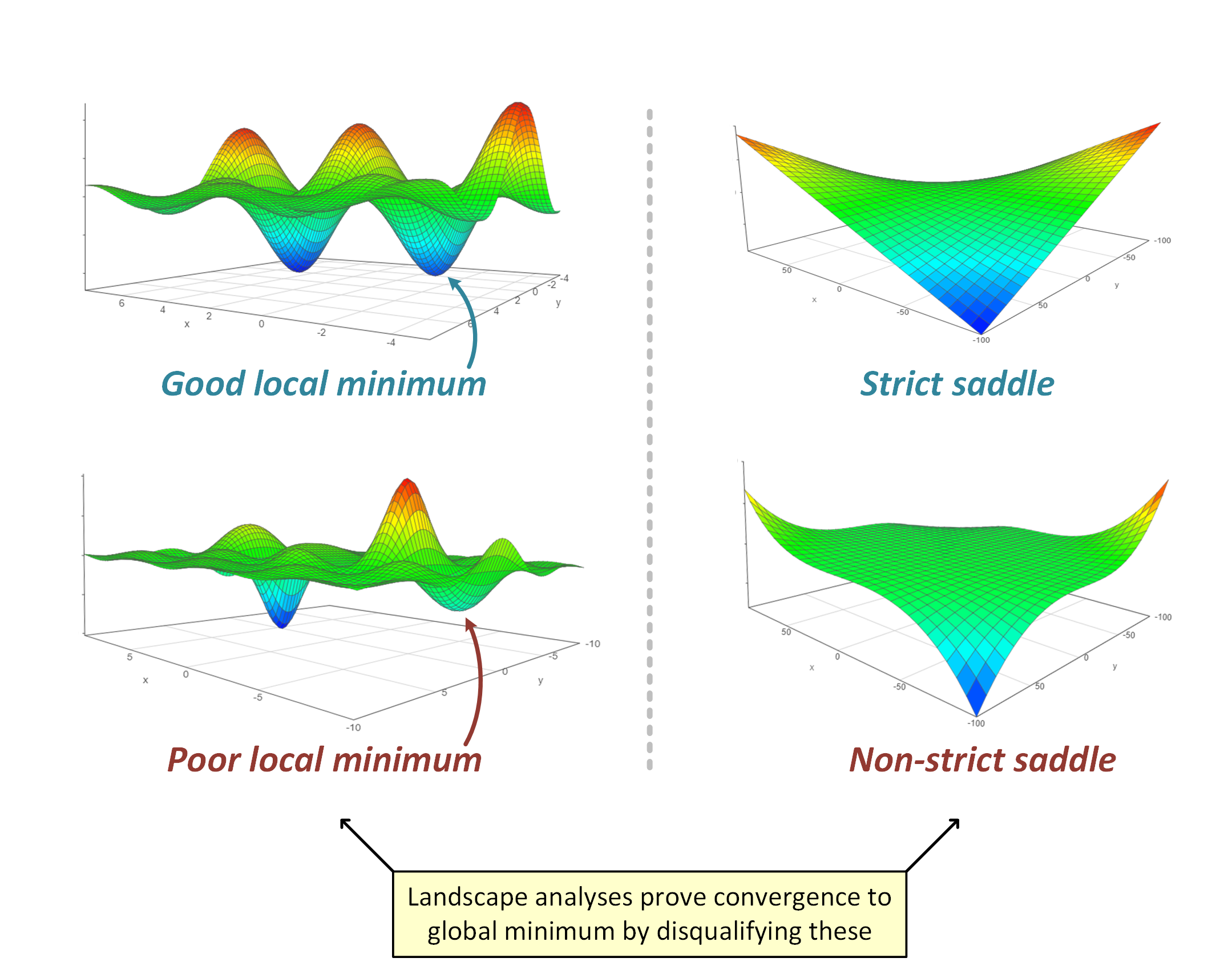
However, it has become clear that the landscape approach (and the Landscape Conjecture) cannot be applied as is to deep (three or more layer) networks, for several reasons. First, deep networks typically induce non-strict saddles (e.g. at the point where all weights are zero, see Kawaguchi 2016). Second, a landscape perspective largely ignores algorithmic aspects that empirically are known to greatly affect convergence with deep networks — for example the type of initialization, or batch normalization. Finally, as I argued in my previous blog post, based upon work with Sanjeev Arora and Elad Hazan, adding (redundant) linear layers to a classic linear model can sometimes accelerate gradient-based optimization, without any gain in expressiveness, and despite introducing non-convexity to a formerly convex problem. Any landscape analysis that relies on properties of critical points alone will have difficulty explaining this phenomenon, as through such lens, nothing is easier to optimize than a convex objective with a single critical point which is the global minimum.
A Way Out?
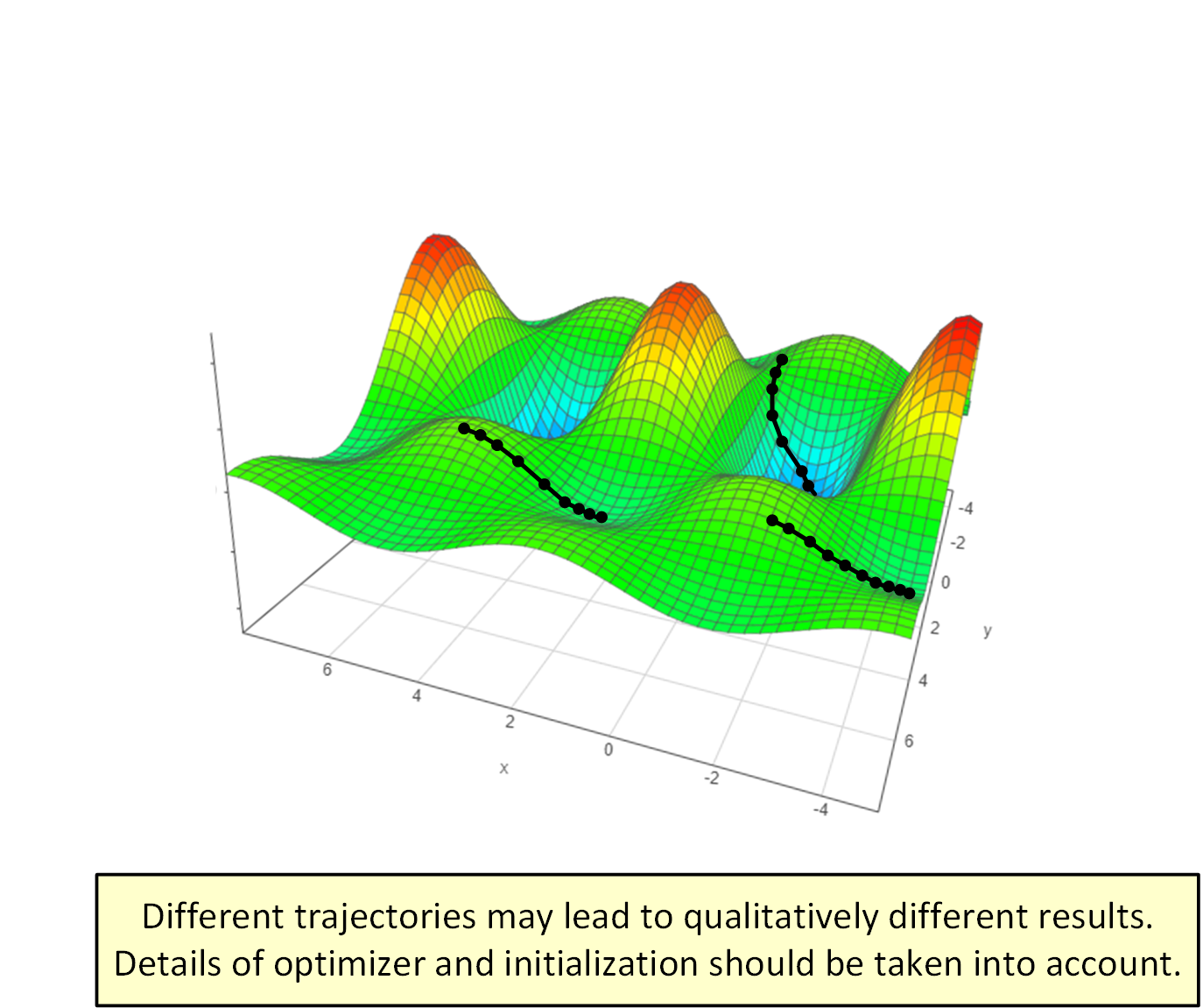
The limitations of the landscape approach for analyzing optimization in deep learning suggest that it may be abstracting away too many important details. Perhaps a more relevant question than “is the landscape graceful?” is “what is the behavior of specific optimizer trajectories emanating from specific initializations?”.
While the trajectory-based approach is seemingly much more burdensome than landscape analyses, it is already leading to notable progress. Several recent papers (e.g. Brutzkus and Globerson 2017; Li and Yuan 2017; Zhong et al. 2017; Tian 2017; Brutzkus et al. 2018; Li et al. 2018; Du et al. 2018; Liao et al. 2018) have adopted this strategy, successfully analyzing different types of shallow models. Moreover, trajectory-based analyses are beginning to set foot beyond the realm of the landscape approach — for the case of linear neural networks, they have successfully established convergence of gradient descent to global minimum under arbitrary depth.
Trajectory-Based Analyses for Deep Linear Neural Networks
Linear neural networks are fully-connected neural networks with linear (no) activation. Specifically, a depth $N$ linear network with input dimension $d_0$, output dimension $d_N$, and hidden dimensions $d_1,d_2,\ldots,d_{N-1}$, is a linear mapping from $\mathbb{R}^{d_0}$ to $\mathbb{R}^{d_N}$ parameterized by $x \mapsto W_N W_{N-1} \cdots W_1 x$, where $W_j \in \mathbb{R}^{d_j \times d_{j-1}}$ is regarded as the weight matrix of layer $j$. Though trivial from a representational perspective, linear neural networks are, somewhat surprisingly, complex in terms of optimization — they lead to non-convex training problems with multiple minima and saddle points. Being viewed as a theoretical surrogate for optimization in deep learning, the application of gradient-based algorithms to linear neural networks is receiving significant attention these days.
To my knowledge, Saxe et al. 2014 were the first to carry out a trajectory-based analysis for deep (three or more layer) linear networks, treating gradient flow (gradient descent with infinitesimally small learning rate) minimizing $\ell_2$ loss over whitened data. Though a very significant contribution, this analysis did not formally establish convergence to global minimum, nor treat the aspect of computational complexity (number of iterations required to converge). The recent work of Bartlett et al. 2018 makes progress towards addressing these gaps, by applying a trajectory-based analysis to gradient descent for the special case of linear residual networks, i.e. linear networks with uniform width across all layers ($d_0=d_1=\cdots=d_N$) and identity initialization ($W_j=I$, $\forall j$). Considering different data-label distributions (which boil down to what they refer to as “targets”), Bartlett et al. demonstrate cases where gradient descent provably converges to global minimum at a linear rate — loss is less than $\epsilon>0$ from optimum after $\mathcal{O}(\log\frac{1}{\epsilon})$ iterations — as well as situations where it fails to converge.
In a new paper with Sanjeev Arora, Noah Golowich and Wei Hu, we take an additional step forward in virtue of the trajectory-based approach. Specifically, we analyze trajectories of gradient descent for any linear neural network that does not include “bottleneck layers”, i.e. whose hidden dimensions are no smaller than the minimum between the input and output dimensions ($d_j \geq \min\{d_0,d_N\}$, $\forall j$), and prove convergence to global minimum, at a linear rate, provided that initialization meets the following two conditions: (i) approximate balancedness — $W_{j+1}^\top W_{j+1} \approx W_j W_j^\top$, $\forall j$; and (ii) deficiency margin — initial loss is smaller than the loss of any rank deficient solution. We show that both conditions are necessary, in the sense that violating any one of them may lead to a trajectory that fails to converge. Approximate balancedness at initialization is trivially met in the special case of linear residual networks, and also holds for the customary setting of initialization via small random perturbations centered at zero. The latter also leads to deficiency margin with positive probability. For the case $d_N=1$, i.e. scalar regression, we provide a random initialization scheme under which both conditions are met, and thus convergence to global minimum at linear rate takes place, with constant probability.
Key to our analysis is the observation that if weights are initialized to be approximately balanced, they will remain that way throughout the iterations of gradient descent. In other words, trajectories taken by the optimizer adhere to a special characterization:
Trajectory Characterization:
\(W_{j+1}^\top(t) W_{j+1}(t) \approx W_j(t) W_j^\top(t), \quad j=1,\ldots,N-1, \quad t=0,1,\ldots\),
which means that throughout the entire timeline, all layers have (approximately) the same set of singular values, and the left singular vectors of each layer (approximately) coincide with the right singular vectors of the layer that follows. We show that this regularity implies steady progress for gradient descent, thereby demonstrating that even in cases where the loss landscape is complex as a whole (includes many non-strict saddle points), it may be particularly well-behaved around the specific trajectories taken by the optimizer.
Conclusion
Tackling the question of optimization in deep learning through the landscape approach, i.e. by analyzing the geometry of the objective independently of the algorithm used for training, is conceptually appealing. However this strategy suffers from inherent limitations, predominantly as it requires the entire objective to be graceful, which seems to be too strict of a demand. The alternative approach of taking into account the optimizer and its initialization, and focusing on the landscape only along the resulting trajectories, is gaining more and more traction. While landscape analyses have thus far been limited to shallow (two layer) models only, the trajectory-based approach has recently treated arbitrarily deep models, proving convergence of gradient descent to global minimum at a linear rate. Much work however remains to be done, as this success covered only linear neural networks. I expect the trajectory-based approach to be key in developing our formal understanding of gradient-based optimization for deep non-linear networks as well.