(Crossposted at CMU ML.)

Traditional wisdom in machine learning holds that there is a careful trade-off between training error and generalization gap. There is a “sweet spot” for the model complexity such that the model (i) is big enough to achieve reasonably good training error, and (ii) is small enough so that the generalization gap - the difference between test error and training error - can be controlled. A smaller model would give a larger training error, while making the model bigger would result in a larger generalization gap, both leading to larger test errors. This is described by the classical U-shaped curve for the test error when the model complexity varies (see Figure 1(a)).

However, it is common nowadays to use highly complex over-parameterized models like deep neural networks. These models are usually trained to achieve near zero error on the training data, and yet they still have remarkable performance on test data. Belkin et al. (2018) characterized this phenomenon by a “double descent” curve which extends the classical U-shaped curve. It was observed that, as one increases the model complexity past the point where it can perfectly fits the training data (i.e., interpolation regime is reached), test error continues to drop! Interestingly, the best test error is often achieved by the largest model, which goes against the classical intuition about the “sweet spot.” The following figure from Belkin et al. (2018) illustrates this phenomenon.

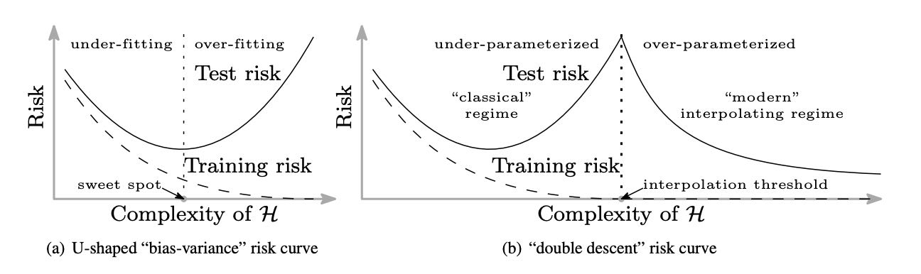
Figure 1. Effect of increased model complexity on generalization: traditional belief vs actual practice.

Consequently one suspects that the training algorithms used in deep learning - (stochastic) gradient descent and its variants - somehow implicitly constrain the complexity of trained networks (i.e., “true number” of parameters), thus leading to a small generalization gap.

Since larger models often give better performance in practice, one may naturally wonder:

How does an infinitely wide net perform?

The answer to this question corresponds to the right end of Figure 1(b). This blog post is about a model that has attracted a lot of attention in the past year: deep learning in the regime where the width - namely, the number of channels in convolutional filters, or the number of neurons in fully-connected internal layers - goes to infinity. At first glance this approach may seem hopeless for both practitioners and theorists: all the computing power in the world is insufficient to train an infinite network, and theorists already have their hands full trying to figure out finite ones. But in math/physics there is a tradition of deriving insights into questions by studying them in the infinite limit, and indeed here too the infinite limit becomes easier for theory.

Experts may recall the connection between infinitely wide neural networks and kernel methods from 25 years ago by Neal (1994) as well as the recent extensions by Lee et al. (2018) and Matthews et al. (2018). These kernels correspond to infinitely wide deep networks whose all parameters are chosen randomly, and only the top (classification) layer is trained by gradient descent. Specifically, if $f(\theta,x)$ denotes the output of the network on input $x$ where $\theta$ denotes the parameters in the network, and $\mathcal{W}$ is an initialization distribution over $\theta$ (usually Gaussian with proper scaling), then the corresponding kernel is \(\mathrm{ker} \left(x,x'\right) = \mathbb{E}_{\theta \sim \mathcal{W}}[f\left(\theta,x\right)\cdot f\left(\theta,x'\right)]\) where $x,x’$ are two inputs.

What about the more usual scenario when all layers are trained? Recently, Jacot et al. (2018) first observed that this is also related to a kernel named neural tangent kernel (NTK), which has the form \(\mathrm{ker} \left(x,x'\right) = \mathbb{E}_{\theta \sim \mathcal{W}}\left[\left\langle \frac{\partial f\left(\theta,x\right)}{\partial \theta}, \frac{\partial f\left(\theta,x'\right)}{\partial \theta}\right\rangle\right].\)

The key difference between the NTK and previously proposed kernels is that the NTK is defined through the inner product between the gradients of the network outputs with respect to the network parameters. This gradient arises from the use of the gradient descent algorithm. Roughly speaking, the following conclusion can be made for a sufficiently wide deep neural network trained by gradient descent:

A properly randomly initialized sufficiently wide deep neural network trained by gradient descent with infinitesimal step size (a.k.a. gradient flow) is equivalent to a kernel regression predictor with a deterministic kernel called neural tangent kernel (NTK).

This was more or less established in the original paper of Jacot et al. (2018), but they required the width of every layer to go to infinity in a sequential order. In our recent paper with Sanjeev Arora, Zhiyuan Li, Ruslan Salakhutdinov and Ruosong Wang, we improve this result to the non-asymptotic setting where the width of every layer only needs to be greater than a certain finite threshold.

In the rest of this post we will first explain how NTK arises and the idea behind the proof of the equivalence between wide neural networks and NTKs. Then we will present experimental results showing how well infinitely wide neural networks perform in practice.

How Does Neural Tangent Kernel Arise?

Now we describe how training an ultra-wide fully-connected neural network leads to kernel regression with respect to the NTK. A more detailed treatment is given in our paper. We first specify our setup. We consider the standard supervised learning setting, in which we are given $n$ training data points ${(x_i,y_i)}_{i=1}^n \subset \mathbb{R}^{d}\times\mathbb{R}$ drawn from some underlying distribution and wish to find a function that given the input $x$ predicts the label $y$ well on the data distribution. We consider a fully-connected neural network defined by $f(\theta, x)$, where $\theta$ is the collection of all the parameters in the network and $x$ is the input. For simplicity we only consider neural network with a single output, i.e., $f(\theta, x) \in \mathbb{R}$, but the generalization to multiple outputs is straightforward.

We consider training the neural network by minimizing the quadratic loss over training data: \(\ell(\theta) = \frac{1}{2}\sum_{i=1}^n (f(\theta,x_i)-y_i)^2.\) Gradient descent with infinitesimally small learning rate (a.k.a. gradient flow) is applied on this loss function $\ell(\theta)$: \(\frac{d \theta(t)}{dt} = - \nabla \ell(\theta(t)),\) where $\theta(t)$ denotes the parameters at time $t$.

Let us define some useful notation. Denote $u_i = f(\theta, x_i)$, which is the network’s output on $x_i$. We let $u=(u_1, \ldots, u_n)^\top \in \mathbb{R}^n$ be the collection of the network outputs on all training inputs. We use the time index $t$ for all variables that depend on time, e.g. $u_i(t), u(t)$, etc. With this notation the training objective can be conveniently written as $\ell(\theta) = \frac12 |u-y|_2^2$.

Using simple differentiation, one can obtain the dynamics of $u(t)$ as follows: (see our paper for a proof)​ \(\frac{du(t)}{dt} = -H(t)\cdot(u(t)-y),\) where $H(t)$ is an $n\times n$ positive semidefinite matrix whose $(i, j)$-th entry is $\left\langle \frac{\partial f(\theta(t), x_i)}{\partial\theta}, \frac{\partial f(\theta(t), x_j)}{\partial\theta} \right\rangle$.

Note that $H(t)$ is the kernel matrix of the following (time-varying) kernel $ker_t(\cdot,\cdot)$ evaluated on the training data: \(ker_t(x,x') = \left\langle \frac{\partial f(\theta(t), x)}{\partial\theta}, \frac{\partial f(\theta(t), x')}{\partial\theta} \right\rangle, \quad \forall x, x' \in \mathbb{R}^{d}.\) In this kernel an input $x$ is mapped to a feature vector $\phi_t(x) = \frac{\partial f(\theta(t), x)}{\partial\theta}$ defined through the gradient of the network output with respect to the parameters at time $t$.

###The Large Width Limit

Up to this point we haven’t used the property that the neural network is very wide. The formula for the evolution of $u(t)$ is valid in general. In the large width limit, it turns out that the time-varying kernel $ker_t(\cdot,\cdot)$ is (with high probability) always close to a deterministic fixed kernel $ker_{\mathsf{NTK}}(\cdot,\cdot)$, which is the neural tangent kernel (NTK). This property is proved in two steps, both requiring the large width assumption:

1. Step 1: Convergence to the NTK at random initialization. Suppose that the network parameters at initialization ($t=0$), $\theta(0)$, are i.i.d. Gaussian. Then under proper scaling, for any pair of inputs $x, x’$, it can be shown that the random variable $ker_0(x,x’)$, which depends on the random initialization $\theta(0)$, converges in probability to the deterministic value $ker_{\mathsf{NTK}}(x,x’)$, in the large width limit.

   (Technically speaking, there is a subtlety about how to define the large width limit. Jacot et al. (2018) gave a proof for the sequential limit where the width of every layer goes to infinity one by one. Later Yang (2019) considered a setting where all widths go to infinity at the same rate. Our paper improves them to the non-asymptotic setting, where we only require all layer widths to be larger than a finite threshold, which is the weakest notion of limit.)

2. Step 2: Stability of the kernel during training. Furthermore, the kernel barely changes during training, i.e., $ker_t(x,x’) \approx ker_0(x,x’)$ for all $t$. The reason behind this is that the weights do not move much during training, namely $\frac{|\theta(t) - \theta(0)|}{|\theta(0)|} \to 0$ as width $\to\infty$. Intuitively, when the network is sufficiently wide, each individual weight only needs to move a tiny amount in order to have a non-negligible change in the network output. This turns out to be true when the network is trained by gradient descent.

Combining the above two steps, we conclude that for any two inputs $x, x’$, with high probability we have \(ker_t(x,x') \approx ker_0(x,x') \approx ker_{\mathsf{NTK}}(x,x'), \quad \forall t.\) As we have seen, the dynamics of gradient descent is closely related to the time-varying kernel $ker_t(\cdot,\cdot)$. Now that we know that $ker_t(\cdot,\cdot)$ is essentially the same as the NTK, with a few more steps, we can eventually establish the equivalence between trained neural network and NTK: the final learned neural network at time $t=\infty$, denoted by $f_{\mathsf{NN}}(x) = f(\theta(\infty), x)$, is equivalent to the kernel regression solution with respect to the NTK. Namely, for any input $x$ we have \(f_{\mathsf{NN}}(x) \approx f_{\mathsf{NTK}}(x) = ker_{\mathsf{NTK}}(x, X)^\top \cdot ker_{\mathsf{NTK}}(X, X)^{-1} \cdot y,\) where $ker_{\mathsf{NTK}}(x, X) = (ker_{\mathsf{NTK}}(x, x_1), \ldots, ker_{\mathsf{NTK}}(x, x_n))^\top \in \mathbb{R}^n$, and $ker_{\mathsf{NTK}}(X, X) $ is an $n\times n$ matrix whose $(i, j)$-th entry is $ker_{\mathsf{NTK}}(x_i, x_j)$.

(In order to not have a bias term in the kernel regression solution we also assume that the network output at initialization is small: $f(\theta(0), x)\approx0$; this can be ensured by e.g. scaling down the initialization magnitude by a large constant, or replicating a network with opposite signs on the top layer at initialization.)

How Well Do Infinitely Wide Neural Networks Perform in Practice?

Having established this equivalence, we can now address the question of how well infinitely wide neural networks perform in practice — we can just evaluate the kernel regression predictors using the NTKs! We test NTKs on a standard image classification dataset, CIFAR-10. Note that for image datasets, one needs to use convolutional neural networks (CNNs) to achieve good performance. Therefore, we derive an extension of NTK, convolutional neural tangent kernels (CNTKs) and test their performance on CIFAR-10. In the table below, we report the classification accuracies of different CNNs and CNTKs:

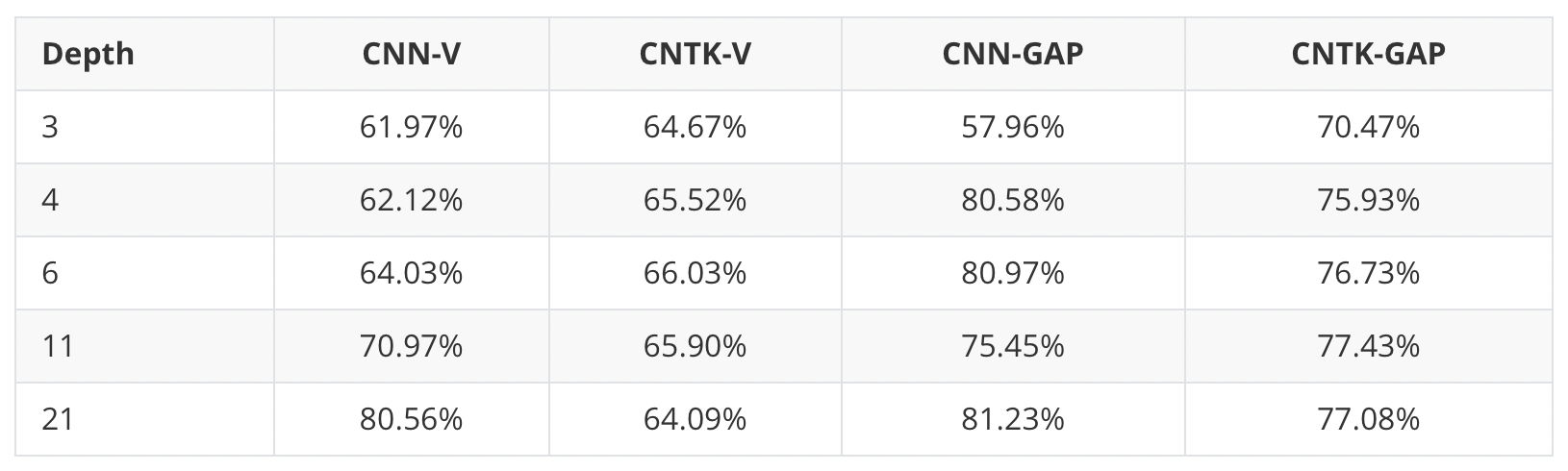
Here CNN-Vs are vanilla practically-wide CNNs (without pooling), and CNTK-Vs are their NTK counterparts. We also test CNNs with global average pooling (GAP), denotes above as CNN-GAPs, and their NTK counterparts, CNTK-GAPs. For all experiments, we turn off batch normalization, data augmentation, etc., and only use SGD to train CNNs (for CNTKs, we use the closed-form formula of kernel regression).

We find that CNTKs are actually very power kernels. The best kernel we find, 11-layer CNTK with GAP, achieves 77.43% classification accuracy on CIFAR-10. This results in a significant new benchmark for performance of a pure kernel-based method on CIFAR-10, being 10% higher than methods reported by Novak et al. (2019). The CNTKs also perform similarly to their CNN counterparts. This means that ultra-wide CNNs can achieve reasonable test performance on CIFAR-10.

It is also interesting to see that the global average pooling operation can significantly increase the classification accuracy for both CNNs and CNTKs. From this observation, we suspect that many techniques that improve the performance of neural networks are in some sense universal, i.e., these techniques might benefit kernel methods as well.

Concluding Thoughts

Understanding the surprisingly good performance of over-parameterized deep neural networks is definitely a challenging theoretical question. Now, at least we have a better understanding of a class of ultra-wide neural networks: they are captured by neural tangent kernels! A hurdle that remains is that the classic generalization theory for kernels is still incapable of giving realistic bounds for generalization. But at least we now know that better understanding of kernels can lead to better understanding of deep nets.

Another fruitful direction is to “translate” different architectures/tricks of neural networks to kernels and to check their practical performance. We have found that global average pooling can significantly boost the performance of kernels, so we hope other tricks like batch normalization, dropout, max-pooling, etc. can also benefit kernels. Similarly, one can try to translate other architectures like recurrent neural networks, graph neural networks, and transformers, to kernels as well.

Our study also shows that there is a performance gap between infinitely wide networks and finite ones. How to explain this gap is an important theoretical question.