TL;DR
A lot was said in this blog (cf. post by Sanjeev) about the importance of studying trajectories of gradient descent (GD) for understanding deep learning. Researchers often conduct such studies by considering gradient flow (GF), equivalent to GD with infinitesimally small step size. Much was learned from analyzing GF over neural networks (NNs), but to what extent do results for GF apply to GD with practical step size? This is an open question in deep learning theory. My student Omer Elkabetz and I investigated it in a recent NeurIPS 2021 spotlight paper. In a nutshell, we found that, although in general an exponentially small step size is required for guaranteeing that GD is well represented by GF, specifically over NNs, a much larger step size can suffice. This allows immediate translation of analyses for GF over NNs to results for GD. The translation bears potential to shed light on both optimization and generalization (implicit regularization) in deep learning, and indeed, we exemplify its use for proving what is, to our knowledge, the first guarantee of random near-zero initialization almost surely leading GD over a deep (three or more layer) NN of fixed size to efficiently converge to global minimum. The remainder of this post provides more details; for the full story see our paper.
GF: a continuous surrogate for GD
Let $f : \mathbb{R}^d \to \mathbb{R}$ be an objective function (e.g. training loss of deep NN) that we would like to minimize via GD with step size $\eta > 0$: [ \boldsymbol\theta_{k + 1} = \boldsymbol\theta_k - \eta \nabla f ( \boldsymbol\theta_k ) ~ ~ ~ \text{for} ~ k = 0 , 1 , 2 , … \qquad \color{green}{\text{(GD)}} ] We may imagine a continuous curve $\boldsymbol\theta : [ 0 , \infty ) \to \mathbb{R}^d$ that passes through the $k$’th GD iterate at time $t = k \eta$. This would imply $\boldsymbol\theta ( t + \eta ) = \boldsymbol\theta ( t ) - \eta \nabla f ( \boldsymbol\theta ( t ) )$, which we can write as $\frac{1}{\eta} ( \boldsymbol\theta ( t + \eta ) - \boldsymbol\theta ( t ) ) = - \nabla f ( \boldsymbol\theta ( t ) )$. In the limit of infinitesimally small step size ($\eta \to 0$), we obtain the following characterization for $\boldsymbol\theta ( \cdot )$: [ \frac{d}{dt} \boldsymbol\theta ( t ) = - \nabla f ( \boldsymbol\theta ( t ) ) ~ ~ ~ \text{for} ~ t \geq 0 . \qquad \color{blue}{\text{(GF)}} ] This differential equation is known as GF, and represents a continuous surrogate for GD.
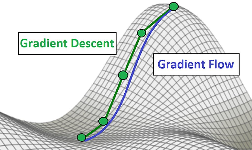
Figure 1: Illustration of GD and its continuous surrogate GF.
GF brings forth the possibility of employing a vast array of continuous mathematical machinery for studying GD. It is for this reason that GF has become a popular model in deep learning theory (see our paper for a long list of works analyzing GF over NNs). There is only one problem: GF assumes infinitesimal step size for GD! This is of course impractical, leading to the following open question $-$ the topic of our work:
Open Question: Does GF over NNs represent GD with practical step size?
GD as numerical integrator for GF
The question of proximity between GF and GD (with positive step size) is closely related to an area of numerical analysis known as numerical integration. There, the motivation is the other way around $-$ given a differential equation $\frac{d}{dt} \boldsymbol\theta ( t ) = \boldsymbol g ( \boldsymbol\theta ( t ) )$ induced by some vector field $\boldsymbol g : \mathbb{R}^d \to \mathbb{R}^d$, the interest lies on a continuous solution $\boldsymbol\theta : [ 0 , \infty ) \to \mathbb{R}^d$, and numerical (discrete) integration algorithms are used for obtaining approximations. A classic numerical integrator, known as Euler’s method, is given by $\boldsymbol\theta_{k + 1} = \boldsymbol\theta_k + \eta \boldsymbol g ( \boldsymbol\theta_k )$ for $k = 0 , 1 , 2 , …$, where $\eta > 0$ is a predetermined step size. With Euler’s method, the goal is for the $k$’th iterate to approximate the sought-after continuous solution at time $k \eta$, meaning $\boldsymbol\theta_k \approx \boldsymbol\theta ( k \eta )$. Notice that when the vector field $\boldsymbol g ( \cdot )$ is chosen to be minus the gradient of an objective function $f : \mathbb{R}^d \to \mathbb{R}$, i.e. $\boldsymbol g ( \cdot ) = - \nabla f ( \cdot )$, the given differential equation is no other than GF, and its numerical integration via Euler’s method yields no other than GD! We can therefore employ known results from numerical integration to bound the distance between GF and GD!
GF matches GD if its trajectory is roughly convex
There exist classic results bounding the approximation error of Euler’s method, but these are too coarse for our purposes. Instead, we invoke a modern result known as “Fundamental Theorem” (cf. Hairer et al. 1993), which implies the following:
Theorem 1: The distance between the GF trajectory $\boldsymbol\theta ( \cdot )$ at time $t$, and iterate $k = t / \eta$ of GD, is upper bounded as:
[ || \boldsymbol\theta ( t ) - \boldsymbol\theta_{k = t / \eta} || \leq \mathcal{O} \Big( e^{- \smallint_0^{~ t} \lambda_- ( t’ ) dt’} t \eta \Big) , ] where $\lambda_- ( t’ ) := \min \left( \lambda_{min} \left( \nabla^2 f ( \boldsymbol\theta ( t’ ) ) \right) , 0 \right)$, i.e. $\lambda_- ( t’ )$ is defined to be the negative part of the minimal eigenvalue of the Hessian on the GF trajectory at time $t’$.
As expected, by using a sufficiently small step size $\eta$, we may ensure that GD is arbitrarily close to GF for arbitrarily long. How small does $\eta$ need to be? For the theorem to guarantee that GD follows GF up to time $t$, we must have $\eta \in \mathcal{O} \big( e^{\smallint_0^{~ t} \lambda_- ( t’ ) dt’} / t \big)$. In particular, $\eta$ must be exponential in $\smallint_0^{~ t} \lambda_- ( t’ ) dt’$, i.e. in the integral of (the negative part of) the minimal Hessian eigenvalue along the GF trajectory (up to time $t$). If the optimized objective $f ( \cdot )$ is convex then Hessian eigenvalues are everywhere non-negative, and therefore $\lambda_- ( \cdot ) \equiv 0$, which means that a moderately small $\eta$ (namely, $\eta \in \mathcal{O} ( 1 / t )$) suffices. If on the other hand $f ( \cdot )$ is non-convex then Hessian eigenvalues may be negative, meaning $\lambda_- ( \cdot )$ may be negative, which in turn implies that $\eta$ may have to be exponentially small. We prove in our paper that there indeed exist cases where an exponentially small step size is unavoidable:
Proposition 1: For any $m > 0$, there exist (non-convex) objectives on which the GF trajectory at time $t$ is not approximated by GD if $\eta \notin \mathcal{O} ( e^{- m t} )$.
Despite this negative result, not all hope is lost. It might be that even though a given objective function is non-convex, specifically over GF trajectories it is “roughly convex,” in the sense that along these trajectories the minimal eigenvalue of the Hessian is “almost non-negative.” This would mean that $\lambda_- ( \cdot )$ is almost non-negative, in which case (by Theorem 1) a moderately small step size suffices in order for GD to track GF!
Trajectories of GF over NNs are roughly convex
Being interested in the match between GF and GD over NNs, we analyzed the geometry of GF trajectories on training losses of NNs with homogeneous activations (e.g. linear, ReLU, leaky ReLU). The following theorem (informally stated) was proven:
Theorem 2: For a training loss of a NN with homogeneous activations, the minimal Hessian eigenvalue is arbitrarily negative across space, but along GF trajectories initialized near zero it is almost non-negative.
Combined with Theorem 1, this theorem suggests that over NNs (with homogeneous activations), in the common regime of near-zero initialization, a moderately small step size for GD suffices in order for it to be well represented by GF! We verify this prospect empirically, demonstrating that in basic deep learning settings, reducing the step size for GD often leads to only slight changes in its trajectory.
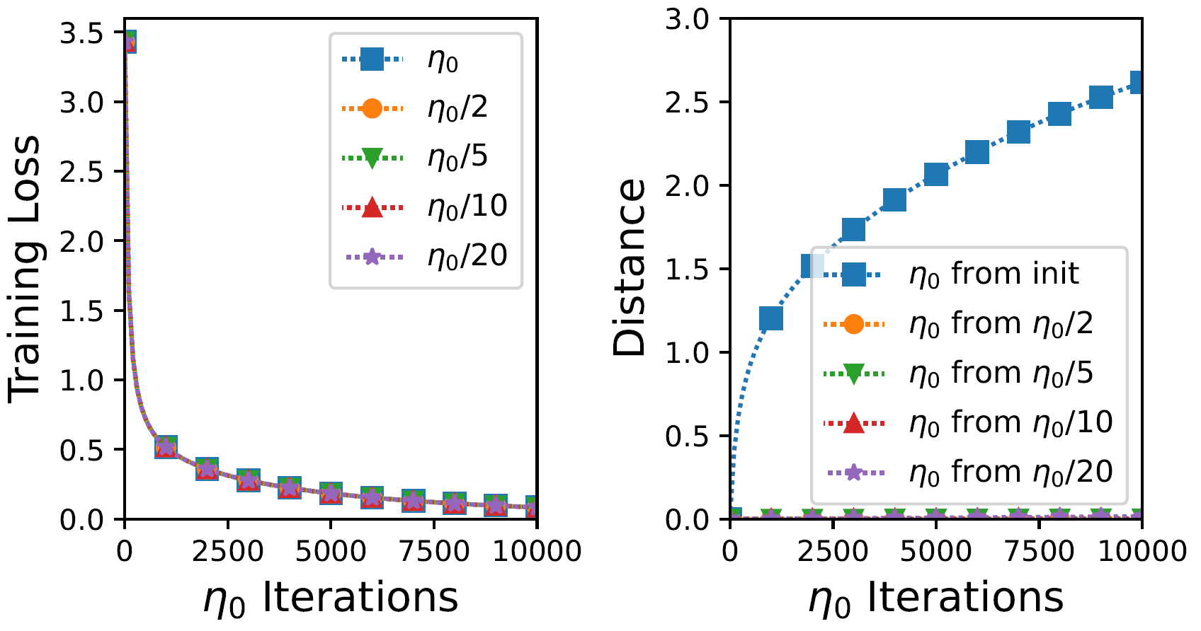
Figure 2: Experiment with NN comparing every iteration of GD with step size $\eta_0 := 0.001$, to every $r$'th iteration of GD with step size $\eta_0 / r$, where $r = 2 , 5 , 10 , 20$. Left plot shows training loss values; right one shows distance (in weight space) of GD with step size $\eta_0$ from initialization, against its distance from runs with smaller step size. Takeaway: reducing step size barely made a difference, suggesting GD was already close to the continuous (GF) limit.
Translating analyses of GF to results for GD
Theorems 1 and 2 together form a tool for automatically translating analyses of GF over NNs to results for GD with practical step size. This means that a vast array of continuous mathematical machinery available for analyzing GF can now be leveraged for formally studying practical NN training! Since analyses of GF over NNs often establish convergence to global minimum and/or characterize the solution found (again, see our paper for long list of examples), the translation we developed bears potential to shed new light on both optimization and generalization (implicit regularization) in deep learning. To demonstrate this point, we analyze GF over arbitrarily deep linear NNs with scalar output, and prove the following result:
Proposition 2: GF over an arbitrarily deep linear NN with scalar output converges to global minimum almost surely (i.e. with probability one) under a random near-zero initialization.
Applying our translation yields an analogous result for GD with practical step size:
Theorem 3: GD over an arbitrarily deep linear NN with scalar output efficiently converges to global minimum almost surely under a random near-zero initialization.
To the best of our knowledge, this is the first guarantee of random near-zero initialization almost surely leading GD over a deep (three or more layer) NN of fixed size to efficiently converge to global minimum!
What about large step size, momentum, stochasticity?
An emerging belief (see our paper for several supporting references) is that for GD over NNs, large step size can be beneficial in terms of generalization. While the large step size regime isn’t necessarily captured by standard GF, recent works (e.g. Barrett & Dherin 2021, Kunin et al. 2021) argue that it is captured by certain modifications of GF. Modifications were also proposed for capturing other aspects of NN training, for example momentum (cf. Su et al. 2016, Wibisono et al. 2016, Franca et al. 2018, Wilson et al. 2021) and stochasticity (see, e.g., Li et al. 2017, Smith et al. 2021, Li et al. 2021). Extending our GF-to-GD translation machinery to account for modifications as above would be very interesting in my opinion. All in all, I believe that in the years to come, the vast knowledge on continuous dynamical systems, and GF in particular, will unravel many mysteries behind deep learning.
Thanks:
I’d like to thank many people with whom I’ve had illuminating discussions on GF vs. GD over NNs.
These include Noah Golowich, Wei Hu, Zhiyuan Li and Kaifeng Lyu.
Special thanks to Govind Menon, who drew my attention to the connection to numerical integration, and of course to Sanjeev, who has been a companion and guide in promoting the “trajectory approach” to deep learning.