In this post we present a high level introduction to evolution and to how we can use mathematical tools such as dynamical systems and Markov chains to model it. Questions about evolution then translate to questions about dynamical systems and Markov chains – some are easy to answer while others point to gaping holes in current techniques in algorithms and optimization. In particular, in this post, we present a setting which captures the evolution of viruses and formulate the question How quickly could evolution happen? This question is not only relevant for the feasibility of drug-design strategies to counter viruses, it also leads to non-trivial questions in computer science.
Just 4 Billion Years…
Starting with the pioneering work of Darwin and Wallace, over the last two centuries there has been tremendous scientific and mathematical advances in our understanding of evolution and how it has shaped diverse and complex life – in a matter of just four billion years. However, unlike physics where the laws seem to be consistent across the universe, evolution is quite complex and its governing dynamics can depend on the context – if we look closely enough, the evolution of life forms such as viruses is quite different from that of humans. Thus, the theory of evolution is not a succinct one, there is vagueness for those who seek mathematical clarity, and, for sure, you should not expect one post to explain all of its various aspects! Instead, we will introduce the basic apparatus of evolution, focus on a concrete setting which has been used to model the evolution of viruses, and ask questions concerning the efficiency of such an evolution.
Evolution in a Nutshell
Abstractly, we can view evolution as nothing but a mechanism (or a meta-algorithm), that takes a population (which is capable of reproducing) as an input and outputs the next generation. At any given time, the population is composed of individuals of different types. As this is all happening in an environment in which resources are limited, who is selected to be a part of the next generation and who is not is determined by the fitness of a type in the environment. The reproduction could be asexual – a simple act of cloning, or sexual – involving the combination of two (or more) individuals to produce offspring. Moreover, during reproduction there could be mutations that transform one type into another. Each of the reproduction, selection or mutation steps could be deterministic or stochastic making evolution either a deterministic or randomized function of the input population.
The size of the population, the number of types, the fitness of each type in the environment, the probabilities of mutation and the starting state are the parameters of the model. Typically, one fixes these parameters and studies how the population evolves over time – whether it reaches a limiting or a steady state and, if so, how this limiting state varies with the parameters of the model and how quickly the limiting state is reached.
After all, evolution without a notion of efficiency is an incomplete theory.
An important and different take on this question is Leslie Valiant’s work on using computational learning theory to understand evolution quantitatively. Finally, as you might have guessed by now, in such generality, evolution encompasses processes which have a priori nothing to do with biology; indeed, evolutionary models have been used to understand many social, economical and cultural phenomena, as described in this book by Nowak.
Populations: Infinite = Dynamical System, Finite = Markov Chain
Given an evolutionary model (which could include stochastic steps), as a first step to understand it we typically assume that the population is infinite and hence all steps are effectively deterministic; we will see an example soon. This allows the evolution of the fraction of each type in the population to be modeled as a deterministic dynamical system from a probability simplex (denoted by $\Delta_m$) to itself; here $m$ is the number of types. However, real populations are finite and often lend themselves to substantial stochastic effects such as random genetic drift. In order to understand their limiting behavior as a function of the population size, we can neither assume that the population is infinite nor ignore stochasticity in the steps in evolution. Hence, Markov chains are appealed to in order to study finite populations. To be concrete, we move on to describing a deterministic and stochastic model for error-prone evolution of an asexual population.
A Deterministic, Infinite Population Model
Consider an infinite population composed of individuals each of who could be one of $m$ types. An individual of type $i$ has a fitness which is specified by a positive integer $a_i,$ and we use a $m \times m$ diagonal matrix $A$ whose $(i,i)$th entry is $a_i$ to capture it. The reproduction is error-prone and this is captured by an $m\times m$ stochastic matrix $Q$ whose $(i,j)$th entry captures the probability that the $j$th type will mutate to the $i$th type during reproduction. In the reproduction stage each type $i$ in the current population produces $a_i$ copies of itself. During reproduction, mutations might occur and in our deterministic model, we assume that one unit of $j$ gives rise to $Q_{i,j}$ fraction of population of $i.$ Since the total mass could become more than one due to reproduction, in the selection stage we normalize the mass so that it is again of unit size.
Thus, the fitness of a type influences its representation in the selected population. Mathematically, we can then track the fraction of each type at step $t$ of the evolution by a vector ${x}^{(t)}\in \Delta_m$ whose evolution is then governed by the dynamical system $ {x}^{(t+1)} = \frac{QA {x}^{(t)}}{\Vert QA {x}^{(t)}\Vert_1}.$ (This is one of the dynamical systems we considered in a previous post.) Thus, the eventual fate of the evolutionary process is not a single type, rather an invariant distribution over types. We saw that when $QA>0$, there is a unique fixed point of this dynamical system; the largest right eigenvalue of $QA.$ Thus, no matter where one starts, this dynamical system converges to this fixed point. Biologically, the corresponding eigenvalue can be shown to be the average fitness of the population which is, in effect, what is being maximized.
How quickly? Well, elementary linear algebra tells us that the rate of convergence of this process is governed by the ratio of the second largest to the largest eigenvalue of $QA.$ Finally, we note that the dynamical system corresponding to a sexually reproducing population is not hard to describe and has been studied recently from an optimization point of view.
A Stochastic, Finite Population Model
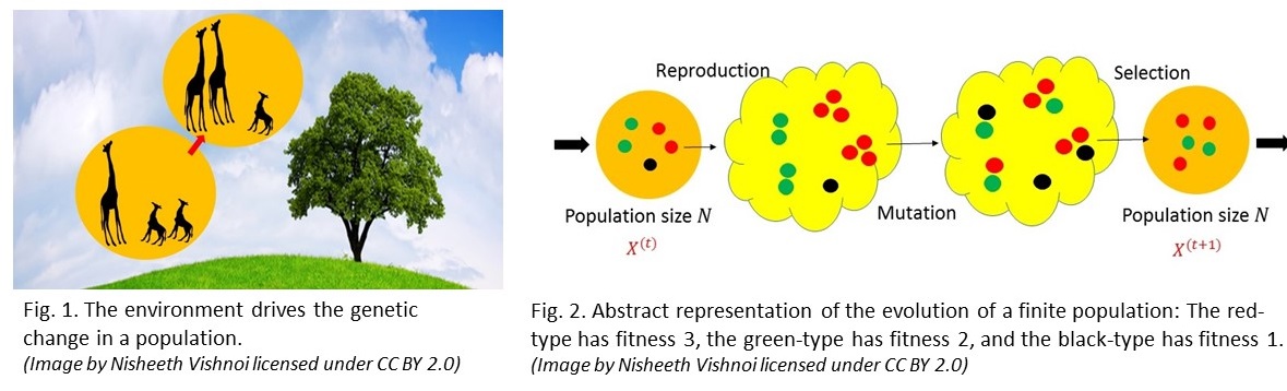
Consider now a stochastic, finite population version of the evolutionary dynamics described above. Here, the population is again assumed to be asexual but now it has a fixed finite size $N.$ After normalization, the composition of the population is again captured by a point in $\Delta_m$ say $ {X}^{(t)}$ at time $t.$ How does one generate ${X^{(t+1)}}$ in this model when the parameters are described by the matrices $Q$ and $A$ as in the infinite population setting? In the reproduction stage, one first replaces an individual of type $i$ in the current population by $a_i$ individuals of type $i$: the total number of individuals of type $i$ in the intermediate population is therefore $a_iN {X_i}^{(t)}$. In the mutation stage, each individual in this intermediate population mutates independently and stochastically according to the matrix $Q.$ Finally, in the selection stage, the population is culled back to size $N$ by sampling $N$ individuals from this intermediate population.
Each of these steps is depicted in Figure 2. Note that stochasticity necessarily means that, even if we initialize the system in the same way, different runs of the chain could produce very different outcomes. The vector $X^{(t+1)}$ then is the normalized frequency vector of the resulting population. The state space of the Markov chain described above has size ${N+m-1}\choose{m-1}.$ When $QA>0,$ this Markov chain is ergodic and, hence, has a unique steady state. However, unlike the deterministic case, this steady state is not apriori easy to compute. Certainly, it has no closed form expression except in the most trivial cases. How do we compute it?
The Mixing Time
The number of states grows roughly like $N^m$ (when $m$ is small compared to $N$) and, even for a small constant $m=40$ and a population of size $10,000$, the number of states is more than $2^{300}$ – more than the number of atoms in the universe! Thus, at best, we can hope to have an algorithm that samples from close to the steady state. In fact, noting that each step of the Markov chain can be implemented efficiently, evolution already provides an algorithm. Its efficiency, however, depends on the time it takes to reach close to steady state – its mixing time. However, in general, there is no way to proclaim that a Markov chain has reached close to its steady state other than providing a bound (along with a proof) on the mixing time. Proving bounds on mixing times of Markov chains is an important area in computer science which interfaces with a variety of other disciplines such as statistics, statistical physics and machine learning; see here. In evolution, however, the mixing time is important beyond computing statistics of samples from the steady state: it tells us how quickly a steady state could be reached. This has biological significance as we will momentarily see in applications of this model to viral evolution.
Viral Evolution and Drug Design: The importance of mixing time
The Markov chain described above has recently found use in modeling RNA viral populations which reproduce asexually and that show strong stochastic behavior (e.g., HIV-1, see here), which in turn has guided drug and vaccine design strategies.
For example, the effective population size of HIV-1 in an infected individual is approximately $10^3-10^6$ not big enough for us to use infinite population models.
Let us see, again at a high-level, how. RNA viruses, due to their primitive copying mechanisms, often undergo mutations during reproduction. Mutations introduce genetic variation and the population at any time is composed of different types – some of them being highly effective (in capturing the host cell) and some not so much. A typical situation to keep in mind is when the number of effective types is a relatively small fraction of $m.$ For the sake of simplicity, let us assume that we are in the setting where each strain mutates to another type with probability $\tau$ during reproduction and remains itself with probability $1-\tau (m-1).$ Thus, as $\tau$ goes from $0$ to $1/m,$ intuitively, in the steady state, the composition of the viral population goes from being concentrated on the effective types to uniformly distributed over all types. The population as a whole is effective if most of its mass in the steady state is concentrated around the effective types and we can declare it dead if it is the latter.
Eigen, in a pioneering work, observed that in fact there is a critical mutation rate called the error threshold around which there is a phase transition – i.e., the virus population changes suddenly from being highly effective to dead.
(This observation was proven formally here). This suggests a strategy to counter viruses: drive their mutation rate past their error threshold! Intriguingly, this strategy is already employed by the body which can produce antibodies that increase the mutation rate. Artificially, this effect can also be accomplished by mutagenic drugs such as ribavirin, see here and here In this setting, knowing the error threshold with high precision is critical: inducing the body with excess mutagenic drugs could have undesired ramifications that lead to complications such as cancer, whereas increasing the rate while keeping it below the threshold can increase the fitness of the virus by allowing it to adapt more effectively, making it more lethal. Computing the error threshold requires the knowledge of the steady state and, thus, is one place where a bound on the mixing time is required. Further, when modeling the effect of a mutagenic drug, the convergence rate determines the minimum required duration of treatment.
If the virus population does not reach its steady state in the lifetime of the infected patient, then what good is that?
To Conclude…
We hope that through this example we have convinced you that efficiency is an important consideration in evolution. Specifically, in the setting we presented, the knowledge of the mixing time of evolutionary Markov chains is a crucial question. Despite its importance, there has been a lack of rigorous mixing time bounds for the full range of parameters, even in the simplest of evolutionary models considered here. Prior work has either ignored mutation, assumed that the model is neutral (i.e., types have the same fitness), or moved to the diffusion limit which requires both mutation and selection pressure to be weak. These bounds apply in some special subcases of evolution and we would like to know mixing time bounds that work for all parameters. In a sequence of results available here, here and here, we have shown that a wide class of evolutionary Markov chains (which includes the one described in this post) can mix quickly for all parameter settings as long as the population is large enough! Further, trying to analyze them has led to new techniques to analyze mixing time of Markov chains and stochastic processes which might be important beyond evolution. We will explain some of these techniques in a subsequent post and continue our discussion, more generally, on evolution viewed from the lens of efficiency.