A big mystery about deep learning is how, in a highly nonconvex loss landscape, gradient descent often finds near-optimal solutions —those with training cost almost zero— even starting from a random initialization. This conjures an image of a landscape filled with deep pits. Gradient descent started at a random point falls easily to the bottom of the nearest pit. In this mental image the pits are disconnected from each other, so there is no way to go from the bottom of one pit to bottom of another without going through regions of high cost.
The current post is about our new paper with Rohith Kuditipudi, Xiang Wang, Holden Lee, Yi Zhang, Wei Hu, Zhiyuan Li and Sanjeev Arora which provides a mathematical explanation of the following surprising phenomenon reported last year.
Mode connectivity (Freeman and Bruna, 2016, Garipov et al. 2018, Draxler et al. 2018) All pairs of low-cost solutions found via gradient descent can actually be connected by simple paths in the parameter space, such that every point on the path is another solution of almost the same cost. In fact the low-cost path connecting two near-optima can be piecewise linear with two line-segments, or a Bezier curve.
See Figure 1 below from Garipov et al. 2018 for an illustration. Solutions A and B have low cost but the line connecting them goes through solutions with high cost. But we can find C of low cost such that paths AC and CB only pass through low-cost region.
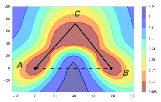
Figure 1 Mode Connectivity. Warm colors represent low loss.
Using a very simple example let us see that this phenomenon is highly counterintuitive. Suppose we’re talking about 2-layer nets with linear activations and a real-valued output. Let the two nets $\theta_A$ and
$\theta_B$ with zero loss be
\(f_1(x) = U_1^\top W_1x \quad f_2(x) = U_2^\top W_2 x\)
respectively where $x, U_1, U_2 \in \Re^n$
and matrices $W_1, W_2$ are $n\times n$. Then the straight line connecting them in parameter space corresponds to nets of the type $(\alpha U_1 + (1-\alpha)U_2)^\top(\alpha W_1 + (1-\alpha)W_2)$ which can be rewritten as
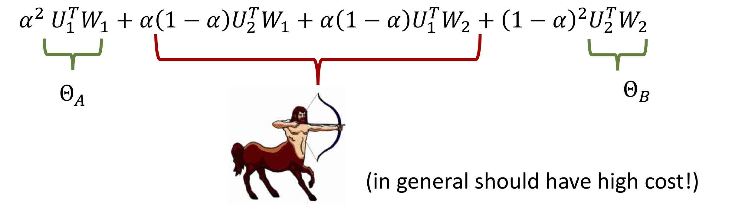
Note that the middle terms correspond to putting the top layer of one net on top of the bottom of the other, which in general is a nonsensical net (reminiscent of a centaur, a mythical half-man half-beast) that in general would be expected to have high loss.
Originally we figured mode connectivity would not be mathematically understood for a long time, because of the seeming difficulty of proving any mathematical theorems about, say, $50$-layer nets trained on ImageNet data, and in particular dealing with such “centaur-like” nets in the interpolation.
Several authors (Freeman and Bruna, 2016, Venturi et al. 2018, Liang et al. 2018, Nguyen et al. 2018, Nguyen et al. 2019) did try to explain the phenomenon of mode connectivity in simple settings (the first of these demonstrated mode connectivity empirically for multi-layer nets). But these explanations only work for very unrealistic 2-layer nets (or multi-layer nets with special structure) which are highly redundant e.g., the number of neurons may have to be larger than the number of training samples.
Our paper starts by clarifying an important point: redundancy with respect to a ground truth neural network is insufficient for mode connectivity, which we show via a simple counterexample sketched below.
Thus to explain mode connectivity for multilayer nets we will need to leverage some stronger property of typical solutions discovered via gradient-based training, as we will see below.
Mode Connectivity need not hold for 2-layer overparametrized nets
We show that the strongest version of mode connectivity (every two minimizers are connected) does not hold even for a simple two-layer setting, where $f(x) = W_2\sigma(W_1x)$, even where the net is vastly overparametrized than it needs to be for the dataset in question.
Theorem For any $h>1$ there exists a data set which is perfectly fitted by a ground truth neural network with $2$ layers and only $2$ hidden neurons, but if we desire to train neural network with $h$ hidden units on this dataset then the set of global minimizers are not connected.
Stability properties of typical nets
Since mode connectivity has been found to hold for a range of architectures and datasets, any explanation probably should only rely upon properties that generically seem to hold for deep net standard training. Our explanation relies upon properties that were discovered in recent years in the effort to understand the generalization properties of deep nets. These properties say that the output of the final net is stable to various kinds of added noise. The properties imply that the loss function does not change much when the net parameters are perturbed; this is informally described as the net being a flat minimum (Hinton and Van Camp 1993).
Our explanation of mode connectivity will involve the following two properties.
Noise stability and Dropout Stability
Dropout was introduced by Hinton et al. 2012: during gradient-based training, one zeroes out the output of $50\%$ of the nodes, and doubles the output of the remaining nodes. The gradient used in the next update is computed for this net. While dropout may not be as popular these days, it can be added to any existing net training without loss of generality. We’ll say a net is “$\epsilon$-dropout stable” if applying dropout to $50\%$ of the nodes increases its loss by at most $\epsilon$. Note that unlike dropout training where nodes are randomly dropped out, in our definition a network is dropout stable as long as there exists a way of dropping out $50\%$ of the nodes that does not increase its loss by too much.
Theorem 1: If two trained multilayer ReLU nets with the same architecture are $\epsilon$-dropout stable, then they can be connected in the loss landscape via a piece-wise linear path in which the number of linear segments is linear in the number of layers, and the loss of every point on the path is at most $\epsilon$ higher than the loss of the two end points.
Noise stability was discovered by Arora et al. ICML18; this was described in a previous blog post. They found that trained nets are very stable to noise injection: if one adds a fairly large Gaussian noise vector to the output of a layer, then this has only a small effect on the output of higher layers. In other words, the network rejects the injected noise. That paper showed that noise stability can be used to prove that the net is compressible. Thus noise stability is indeed a form of redundancy in the net.
In the new paper we show that a minor variant of the noise stability property (which we empirically find to still hold in trained nets) implies dropout stability. More importantly, solutions satisfying this property can be connected using a piecewise linear path with at most $10$ segments.
Theorem 2: If two trained multilayer ReLU nets with the same architecture are $\epsilon$-noise stable, then they can be connected in the loss landscape via a piece-wise linear path with at most 10 segments, and the loss of every point on the path is at most $\epsilon$ higher than the loss of the two end points.
Proving mode connectivity for dropout-stable nets
We exhibit the main ideas by proving mode connectivity for fully connected nets that are dropout-stable, meaning training loss is stable to dropping out $50\%$ of the nodes.
Let $W_1,W_2,…,W_p$ be the weight matrices of the neural network, so the function that is computed by the network is $f(x) = W_p\sigma(\cdots \sigma(W_2(\sigma(W_1x)))\cdots)$. Here $\sigma$ is the ReLU activation (our result in this section works for any activations). We use $\theta = (W_1,W_2,…,W_p)\in \Theta$ to denote the parameters for the neural network. Given a set of data points $(x_i,y_i)~i=1,2,…,n$, the empirical loss $L$ is just an average of the losses for the individual samples $L(\theta) = \frac{1}{n}\sum_{i=1}^n l(y_i, f_\theta(x_i))$. The function $l(y, \hat{y})$ is a loss function that is convex in the second parameter (popular loss functions such as cross-entropy or mean-squared-error are all in this category).
Using this notation, Theorem 1 can be restated as:
Theorem 1 (restated) Let $\theta_A$ and $\theta_B$ be two solutions that are both $\epsilon$-dropout stable, then there exists a path $\pi:[0,1]\to \Theta$ such that $\pi(0) = \theta_A$, $\pi(1) = \theta_B$ and for any $t\in(0,1)$ the loss $L(\pi(t)) \le \max{L(\theta_A), L(\theta_B)} + \epsilon$.
To prove this theorem, the major step is to connect a network with its dropout version where half of the neurons are not used (see next part). Then intuitively it is not too difficult to connect two dropout versions as they both have a large number of inactive neurons.
As we discussed before, directly interpolating between two networks may not work as it give rise to centaur-like networks. A key idea in this simpler theorem is that each linear segment in the path involves varying the parameters of only one layer, which allows careful control of this issue. (Proof of Theorem 2 is more complicated because the number of layers in the net are allowed to exceed the number of path segments.)
As a simple example, we show how to connect a 3-layer neural network with its dropout version. (The same idea can be easily extended to more layers by a simple induction on number of layers.) Assume without loss of generality that we are going to dropout the second half of neurons for both hidden layers. For the weight matrices $W_3, W_2, W_1$, we will write them in block form: $W_3$ is a $1\times 2$ block matrix $W_3 = [L_3, R_3]$, $W_2$ is a $2\times 2$ block matrix $W_2 = \left[L_2, C_2; D_2, R_2 \right]$, and $W_1$ is a $2\times 1$ block matrix $W_1 = \left[L_1; B_1\right]$ (here ; represents the end of a row). The dropout stable property implies that the networks with weights $(W_3, W_2, W_1)$, $(2[L_3, 0], W_2, W_1)$, $([2L_3, 0], [2L_2, 0; 0, 0], W_1)$ all have low loss (these weights correspond to the cases of no dropout, dropout only applied to the top hidden layer and dropout applied to both hidden layers). Note that the final set of weights $([2L_3, 0], [2L_2, 0; 0, 0], W_1)$ is equivalent to $([2L_3, 0], [2L_2, 0; 0, 0], [L_1; 0])$ as the output from the $B_1$ part of $W_1$ has no connections. The path we construct is illustrated in Figure 2 below: As a simple example, we show how to connect a 3-layer neural network with its dropout version. (The same idea can be easily extended to more layers by a simple induction on number of layers.) Assume without loss of generality that we are going to dropout the second half of neurons for both hidden layers. For the weight matrices $W_3, W_2, W_1$, we will write them in block form: $W_3$ is a $1\times 2$ block matrix $W_3 = [L_3, R_3]$, $W_2$ is a $2\times 2$ block matrix $W_2 = \left[L_2, C_2; D_2, R_2 \right]$, and $W_1$ is a $2\times 1$ block matrix $W_1 = \left[L_1; B_1\right]$ (here ; represents the end of a row). The dropout stable property implies that the networks with weights $(W_3, W_2, W_1)$, $(2[L_3, 0], W_2, W_1)$, $([2L_3, 0], [2L_2, 0; 0, 0], W_1)$ all have low loss (these weights correspond to the cases of no dropout, dropout only applied to the top hidden layer and dropout applied to both hidden layers). Note that the final set of weights $([2L_3, 0], [2L_2, 0; 0, 0], W_1)$ is equivalent to $([2L_3, 0], [2L_2, 0; 0, 0], [L_1; 0])$ as the output from the $B_1$ part of $W_1$ has no connections. The path we construct is illustrated in Figure 2 below:
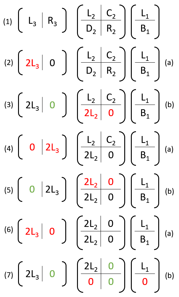
Figure 2 Path from a 3-layer neural network to its dropout version.
We use two types of steps to construct the path: (a) Since the loss function is convex in the weight of the top layer, we can interpolate between two different networks that only differ in top layer weights; (b) if a set of neurons already has 0 output weights, then we can set its input weights arbitrarily.
Figure 2 shows how to alternate between these two types of steps to connect a 3-layer network to its dropout version. The red color highlights weights that have changed. In the case of type (a) steps, the red color only appears in the top layer weights; in the case of type (b) steps, the 0 matrices highlighted by the green color are the 0 output weights, where because of these 0 matrices setting the red blocks to any matrix will not change the output of the neural network.
The crux of this construction appears in steps (3) and (4). When we are going from (2) to (3), we changed the bottom rows of $W_2$ from $[D_2, R_2]$ to $[2L_2, 0]$. This is a type (b) step, and because currently the top-level weight is $[2L_3, 0]$, changing the bottom row of $W_2$ has no effect on the output of the neural network. However, making this change allows us to do the interpolation between (3) and (4), as now the two networks only differ in the top layer weights. The loss is bounded because the weights in (3) are equivalent to $(2[L_3, 0], W_2, W_1)$ (weights with dropout applied to top hidden layer), and the weights in (4) are equivalent to $([2L_3, 0], [2L_2, 0; 0, 0], W_1)$ (weights with dropout applied to both hidden layers). The same procedure can be repeated if the network has more layers.
The number of line segments in the path is linear in the number of layers. As mentioned, the paper also gives stronger results assuming noise stability, where we can actually consruct a path with constant number of line segments.
Conclusions
Our results are a first-cut explanation for how mode connectivity can arise in realistic deep nets. Our methods do not answer all mysteries about mode connectivity. In particular, in many cases (especially when the number of parameters is not as large) the solutions found in practice are not as robust as we require in our theorems (either in terms of dropout stability or noise stability), yet empirically it is still possible to find simple paths connecting the solutions. Are there other properties satisfied by these solutions that allow them to be connected? Also, our results can be extended to convolutional neural networks via channel-wise dropout, where one randomly turn off half of the channels (this was considered before in Thompson et al. 2015,Keshari et al.2018). While it is possible to train networks that are robust to channel-wise dropout, standard networks or even the ones trained with standard dropout do not satisfy this property.
It would also be interesting to utilize the insights into the landscape given by our explanation to design better training algorithms.