Deep learning holds many mysteries for theory, as we have discussed on this blog. Lately many ML theorists have become interested in the generalization mystery: why do trained deep nets perform well on previously unseen data, even though they have way more free parameters than the number of datapoints (the classic “overfitting” regime)? Zhang et al.’s paper Understanding Deep Learning requires Rethinking Generalization played some role in bringing attention to this challenge. Their main experimental finding is that if you take a classic convnet architecture, say Alexnet, and train it on images with random labels, then you can still achieve very high accuracy on the training data. (Furthermore, usual regularization strategies, which are believed to promote better generalization, do not help much.) Needless to say, the trained net is subsequently unable to predict the (random) labels of still-unseen images, which means it doesn’t generalize. The paper notes that the ability to fit a classifier to data with random labels is also a traditional measure in machine learning called Rademacher complexity (which we will discuss shortly) and thus Rademacher complexity gives no meaningful bounds on sample complexity. I found this paper entertainingly written and recommend reading it, despite having given away the punchline. Congratulations to the authors for winning best paper at ICLR 2017.

But I would be remiss if I didn’t report that at the Simons Institute Semester on theoretical ML in spring 2017 generalization theory experts expressed unhappiness about this paper, and especially its title. They felt that similar issues had been extensively studied in context of simpler models such as kernel SVMs (which, to be fair, is clearly mentioned in the paper). It is trivial to design SVM architectures with high Rademacher complexity which nevertheless train and generalize well on real-life data. Furthermore, theory was developed to explain this generalization behavior (and also for related models like boosting). On a related note, several earlier papers of Behnam Neyshabur and coauthors (see this paper and for a full account, Behnam’s thesis) had made points fairly similar to Zhang et al. pertaining to deep nets.

But regardless of such complaints, we should be happy about the attention brought by Zhang et al.’s paper to a core theory challenge. Indeed, the passionate discussants at the Simons semester themselves banded up in subgroups to address this challenge: these resulted in papers by Dzigaite and Roy, then Bartlett, Foster, and Telgarsky and finally Neyshabur, Bhojapalli, MacAallester, Srebro. (The latter two were presented at NIPS’17 this week.)

Before surveying these results let me start by suggesting that some of the controversy over the title of Zhang et al.’s paper stems from some basic confusion about whether or not current generalization theory is prescriptive or merely descriptive. These confusions arise from the standard treatment of generalization theory in courses and textbooks, as I discovered while teaching the recent developments in my graduate seminar.

Prescriptive versus descriptive theory

To illustrate the difference, consider a patient who says to his doctor: “Doctor, I wake up often at night and am tired all day.”

Doctor 1 (without any physical examination): “Oh, you have sleep disorder.”

I call such a diagnosis descriptive, since it only attaches a label to the patient’s problem, without giving any insight into how to solve the problem. Contrast with:

Doctor 2 (after careful physical examination): “A growth in your sinus is causing sleep apnea. Removing it will resolve your problems.”

Such a diagnosis is prescriptive.

Generalization theory: descriptive or prescriptive?

Generalization theory notions such as VC dimension, Rademacher complexity, and PAC-Bayes bound, consist of attaching a descriptive label to the basic phenomenon of lack of generalization. They are hard to compute for today’s complicated ML models, let alone to use as a guide in designing learning systems.

Recall what it means for a hypothesis/classifier $h$ to not generalize. Assume the training data consists of a sample $S = {(x_1, y_1), (x_2, y_2),\ldots, (x_m, y_m)}$ of $m$ examples from some distribution ${\mathcal D}$. A loss function $\ell$ describes how well hypothesis $h$ classifies a datapoint: the loss $\ell(h, (x, y))$ is high if the hypothesis didn’t come close to producing the label $y$ on $x$ and low if it came close. (To give an example, the regression loss is $(h(x) -y)^2$.) Now let us denote by $\Delta_S(h)$ the average loss on samplepoints in $S$, and by $\Delta_{\mathcal D}(h)$ the expected loss on samples from distribution ${\mathcal D}$. Training generalizes if the hypothesis $h$ that minimises $\Delta_S(h)$ for a random sample $S$ also achieves very similarly low loss $\Delta_{\mathcal D}(h)$ on the full distribution. When this fails to happen, we have:

Lack of generalization: $\Delta_S(h) \ll \Delta_{\mathcal D}(h) \qquad (1). $

In practice, lack of generalization is detected by taking a second sample (“held out set”) $S_2$ of size $m$ from ${\mathcal D}$. By concentration bounds expected loss of $h$ on this second sample closely approximates $\Delta_{\mathcal D}(h)$, allowing us to conclude

Generalization Theory: Descriptive Parts

Let’s discuss Rademacher complexity, which I will simplify a bit for this discussion. (See also scribe notes of my lecture.) For convenience assume in this discussion that labels and loss are $0,1$, and assume that the badly generalizing $h$ predicts perfectly on the training sample $S$ and is completely wrong on the heldout set $S_2$, meaning

$\Delta_S(h) - \Delta_{S_2}(h) \approx - 1 \qquad (3)$

Rademacher complexity concerns the following thought experiment. Take a single sample of size $2m$ from $\mathcal{D}$, split it into two and call the first half $S$ and the second $S_2$. Flip the labels of points in $S_2$. Now try to find a classifier $C$ that best describes this new sample, meaning one that minimizes $\Delta_S(h) + 1- \Delta_{S_2}(h)$. This expression follows since flipping the label of a point turns good classification into bad and vice versa, and thus the loss function for $S_2$ is $1$ minus the old loss. We say the class of classifiers has high Rademacher complexity if with high probability this quantity is small, say close to $0$.

But a glance at (3) shows that it implies high Rademacher complexity: $S, S_2$ were random samples of size $m$ from $\mathcal{D}$, so their combined size is $2m$, and when generalization failed we succeeded in finding a hypothesis $h$ for which $\Delta_S(h) + 1- \Delta_{S_2}(h)$ is very small.

In other words, returning to our medical analogy, the doctor only had to hear “Generalization didn’t happen” to pipe up with: “Rademacher complexity is high.” This is why I call this result descriptive.

The VC dimension bound is similarly descriptive. VC dimension is defined to be at least $k +1$ if there exists a set of size $k$ such that the following is true. If we look at all possible classifiers in the class, and the sequence of labels each gives to the $k$ datapoints in the sample, then we can find all possible $2^{k}$ sequences of $0$’s and $1$’s.

If generalization does not happen as in (2) or (3) then this turns out to imply that VC dimension is at least around $\epsilon m$ for some $\epsilon >0$. The reason is that the $2m$ data points were split randomly into $S, S_2$, and there are $2^{2m}$ such splittings. When the generalization error is $\Omega(1)$ this can be shown to imply that we can achieve $2^{\Omega(m)}$ labelings of the $2m$ datapoints using all possible classifiers. Now the classic Sauer’s lemma (see any lecture notes on this topic, such as Schapire’s) can be used to show that VC dimension is at least $\epsilon m/\log m$ for some constant $\epsilon>0$.

Thus again, the doctor only has to hear “Generalization didn’t happen with sample size $m$” to pipe up with: “VC dimension is higher than $\Omega(m/log m)$.”

One can similarly show that PAC-Bayes bounds are also descriptive, as you can see in scribe notes from my lecture.

Why do students get confused and think that such tools of generalization theory gives some powerful technique to guide design of machine learning algorithms?

Answer: Probably because standard presentation in lecture notes and textbooks seems to pretend that we are computationally-omnipotent beings who can compute VC dimension and Rademacher complexity and thus arrive at meaningful bounds on sample sizes needed for training to generalize. While this may have been possible in the old days with simple classifiers, today we have complicated classifiers with millions of variables, which furthermore are products of nonconvex optimization techniques like backpropagation. The only way to actually lowerbound Rademacher complexity of such complicated learning architectures is to try training a classifier, and detect lack of generalization via a held-out set. Every practitioner in the world already does this (without realizing it), and kudos to Zhang et al. for highlighting that theory currently offers nothing better.

Toward a prescriptive generalization theory: the new papers

In our medical analogy we saw that the doctor needs to at least do a physical examination to have a prescriptive diagnosis. The authors of the new papers intuitively grasp this point, and try to identify properties of real-life deep nets that may lead to better generalization. Such an analysis (related to “margin”) was done for simple 2-layer networks couple decades ago, and the challenge is to find analogs for multilayer networks. Both Bartlett et al. and Neyshabur et al. hone in on stable rank of the weight matrices of the layers of the deep net. These can be seen as an instance of a “flat minimum” which has been discussed in neural nets literature for many years. I will present my take on these results as well as some improvements in a future post. Note that these methods do not as yet give any nontrivial bounds on the number of datapoints needed for training the nets in question.

Dziugaite and Roy take a slightly different tack. They start with McAllester’s 1999 PAC-Bayes bound, which says that if the algorithm’s prior distribution on the hypotheses is $P$ then for every posterior distributions $Q$ (which could depend on the data) on the hypotheses the generalization error of the average classifier picked according to $Q$ is upper bounded as follows where $D()$ denotes KL divergence:

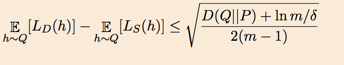
This allows upperbounds on generalization error (specifically, upperbounds on number of samples that guarantee such an upperbound) by proceeding as in Langford and Caruana’s old paper where $P$ is a uniform gaussian, and $Q$ is a noised version of the trained deep net (whose generalization we are trying to explain). Specifically, if $w_{ij}$ is the weight of edge ${i, j}$ in the trained net, then $Q$ consists of adding a gaussian noise $\eta_{ij}$ to weight $w_{ij}$. Thus a random classifier according to $Q$ is nothing but a noised version of the trained net. Now we arrive at the crucial idea: Use nonconvex optimization to find a choice for the variance of $\eta_{ij}$ that balances two competing criteria: (a) the average classifier drawn from $Q$ has training error not much more than the original trained net (again, this is a quantification of the “flatness” of the minimum found by the optimization) and (b) the right hand side of the above expression is as small as possible. Assuming (a) and (b) can be suitably bounded, it follows that the average classifier from Q works reasonably well on unseen data. (Note that this method only proves generalization of a noised version of the trained classifier.)

Applying this method on simple fully-connected neural nets trained on MNIST dataset, they can prove that the method achieves error $17$ percent error on MNIST (whereas the actual error is much lower at 2-3 percent). Hence the title of their paper, which promises nonvacuous generalization bounds. What I find most interesting about this result is that it uses the power of nonconvex optimization (harnessed above to find a suitable noised distribution $Q$) to cast light on one of the metaquestions about nonconvex optimization, namely, why does deep learning not overfit!