Convex functions are simple — they usually have only one local minimum. Non-convex functions can be much more complicated. In this post we will discuss various types of critical points that you might encounter when you go off the convex path. In particular, we will see in many cases simple heuristics based on gradient descent can lead you to a local minimum in polynomial time.
Various Types of Critical Points

To minimize the function $f:\mathbb{R}^n\to \mathbb{R}$, the most popular approach is to follow the opposite direction of the gradient $\nabla f(x)$ (for simplicity, all functions we talk about are infinitely differentiable), that is,
\[y = x - \eta \nabla f(x),\]Here $\eta$ is a small step size. This is the gradient descent algorithm.
Whenever the gradient $\nabla f(x)$ is nonzero, as long as we choose a small enough $\eta$, the algorithm is guaranteed to make local progress. When the gradient $\nabla f(x)$ is equal to $\vec{0}$, the point is called a critical point, and gradient descent algorithm will get stuck. For (strongly) convex functions, there is a unique critical point that is also the global minimum.
However, for non-convex functions, just having the gradient to be $\vec{0}$ is not good enough. A simple example is the function
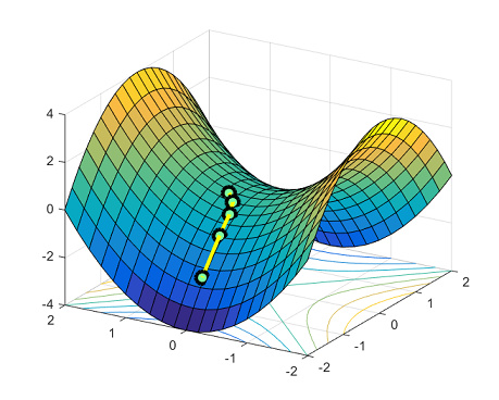
\[y = x_1^2 - x_2^2.\]At $x = (0,0)$, the gradient is $\vec{0}$, but it is clearly not a local minimum as $x = (0, \epsilon)$ has smaller function value. The point $(0,0)$ is called a saddle point of this function.
To distinguish these cases we need to consider the second order derivative $\nabla^2 f(x)$ — an $n\times n$ matrix (usually known as the Hessian) whose $i,j$-th entry is equal to $\frac{\partial^2}{\partial x_i \partial x_j} f(x)$. When the Hessian is positive definite (which means $u^\top\nabla^2 f(x) u > 0$ for any $u\ne 0$), by second order Taylor’s expansion for any direction $u$ \(f(x + \eta u) \approx f(x) + \frac{\eta^2}{2} u^\top\nabla^2 f(x) u > f(x),\) therefore $x$ must be a local minimum. Similarly, when the Hessian is negative definite, the point is a local maximum; when the Hessian has both positive and negative eigenvalues, the point is a saddle point.
It is believed that for many problems including learning deep nets, almost all local minimum have very similar function value to the global optimum, and hence finding a local minimum is good enough. However, it is NP-hard to even find a local minimum (see Discussions in Anandkumar, Ge 2006). Many popular optimization techniques in practice are first order optimization algorithms: they only look at the gradient information, and never explicitly compute the Hessian. Such algorithms may get stuck at saddle points.
In the rest of the post, we will first see that getting stuck at saddle points is a very realistic possibility since most natural objective functions have exponentially many saddle points. We will then discuss how optimization algorithms can try to escape from saddle points.
Symmetry and Saddle Points
Many learning problems can be abstracted as searching for $k$ distinct components (sometimes called features, centers,…). For example, in the clustering problem, there are $n$ points, and we are searching for $k$ components that minimizes the sum of distances of points to their nearest center. In a two-layer neural network, we try to find a network with $k$ distinct neurons at the middle layer. In my previous post I talked about tensor decomposition, which also looks for $k$ distinct rank-1 components.
A popular way to solve these problems is to design an objective function: let $x_1, x_2, \ldots, x_k \in \mathbb{R}^n$ denote the desired centers and let objective function $f(x_1,…,x_k)$ measure the quality of the solution. The function is minimized when the vectors $x_1,x_2,…,x_k$ are the $k$ components that we are looking for.
A natural reason why any such problem is inherently non-convex is permutation symmetry. For instance, if we swap the order of first and second component, the solutions are equivalent. Namely, \(f(x_1,x_2,...,x_k) = f(x_2, x_1,...,x_k).\)
However, if we take the average of this solution, we will end up with the solution $\frac{x_1+x_2}{2}, \frac{x_1+x_2}{2}, x_3,…,x_k$, which is not equivalent! If the original solution is optimal this average is likely to be suboptimal. Therefore the objective function cannot be convex because for convex functions, average of optimal solutions is still optimal.

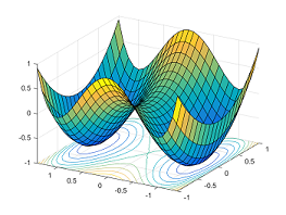
There are exponentially many globally optimal solutions that are all permutations of the same solution. Saddle points arise naturally on the paths that connect these isolated local minima. The figure below shows the function $y = x_1^4-2x_1^2 + x_2^2$: between two symmetric local min $(-1,0)$ and $(1,0)$, the point $(0,0)$ is a saddle point.

Escaping from Saddle Points
In order to optimize these non-convex functions with many saddle points, optimization algorithms need to make progress even at (or near) saddle points. The simplest way to do this is by using the second order Taylor’s expansion:
\[f(y) \approx f(x) + \left<\nabla f(x), y-x\right>+\frac{1}{2} (y-x)^\top \nabla^2 f(x) (y-x).\]If the gradient $\nabla f(x)$ is $\vec{0}$, we can still hope to find a vector $u$ where $u^\top \nabla^2 f(x) u < 0$. This way if we let $y = x+\eta u$, the function value of $f(y)$ is likely to be smaller. Many optimization algorithms such as trust region algorithms and cubic regularization use this idea, and they can escape from saddle points in polynomial time for nice functions.
Strict Saddle Functions
As we discussed, in general it is NP-hard to find a local minimum and many algorithms may get stuck at a saddle point. How many steps do we need to escape from a saddle point? This is related to how well-behaved the saddle points are. Intuitively, a saddle point $x$ is well-behaved, if there is a direction $u$ such that the second order term $u^\top \nabla^2 f(x) u$ is significantly smaller than 0 — geometrically this means there is a steep direction where the function value decreases. To quantify this, my paper with Furong Huang, Chi Jin and Yang Yuan introduced the notion of strict saddle functions (also known as “ridable” function in Sun et al. 2015)
A function $f(x)$ is strict saddle if all points $x$ satisfy at least one of the following
- Gradient $\nabla f(x)$ is large.
- Hessian $\nabla^2 f(x)$ has a negative eigenvalue that is bounded away from 0.
- Point $x$ is near a local minimum.
Essentially, the local region of every point $x$ looks like one of the following pictures:

For such functions, trust region algorithms and cubic regularization can find a local minimum efficiently.
Theorem(Informal) There are polynomial time algorithms that can find a local minimum of strict saddle functions.
What functions are strict saddle? Ge et al. 2015 showed a tensor decomposition problem is strict saddle. Sun et al. 2015 observed that problems like complete dictionary learning, phase retrieval are also strict saddle.
First Order Method to Escape from Saddle Points
Trust region algorithms are very powerful. However they need to compute the second order derivative of the objective function, which is often too expensive in practice. If the algorithm can only access the gradient of the function, is it still possible to escape from saddle points?
This might seem hard as the gradient at a saddle point is $\vec{0}$ and does not give us any information. However, the key observation here is saddle points are very unstable: if we put a ball on a saddle point, then slightly perturb it, the ball is likely to fall! Of course we need to make this intuition formal in higher dimensions, as naively to find the direction to fall it seems to require computing the smallest eigenvector of the Hessian matrix.
To formalize this intuition we will try use a noisy gradient descent
$y = x - \eta \nabla f(x) + \epsilon.$
Here $\epsilon$ is a noise vector that has mean $0$. This additional noise is going to deliver the initial nudge that makes the ball fall along the slope.
In fact, often it is much cheaper to compute a noisy gradient than the true gradient — this is the key idea in stochastic gradient , and a large body of work shows that the noise does not interfere with convergence for convex optimization. For non-convex optimization, intuitively people believed the inherent noise helps in convergence because it pushes the current point away from saddle points. It’s not a bug, it’s a feature!

Previously, there were no good upper bound known on the number of iterations needed to escape saddle points and arrive at a local minimum. In Ge et al. 2015, we show
Theorem(Informal) Noisy gradient descent can find a local minimum of strict saddle functions in polynomial time.
The polynomial dependency on the dimension $n$ and the smallest eigenvalue of the Hessian are fairly high and not very practical. It is an open problem to find the optimal convergence rate for strict saddle problems.
A recent subsequent paper by Lee et al. showed even without adding noise, gradient descent will not converge to any strict saddle point if the initial point is chosen randomly. However their result relies on the Stable Manifold Theorem from dynamical systems theory, which inherently does not provide any upperbound on the number of steps.
Beyond Simple Saddle Points
We have seen algorithms that can handle (simple) saddle points. However, non-convex problems can have much more complicated landscapes that involve degenerate saddle points — points whose Hessian is positive semidefinite and have 0 eigenvalues. Such degenerate structure often indicates a complicated saddle point (such as a monkey saddle, Figure (a)) or a set of connected saddle points (Figures (b)(c)). In Anandkumar, Ge 2016 we gave an algorithm that can deal with some of these degenerate saddle points.

The landscapes of non-convex functions can be very complicated, and there are still many open problems. What other functions are strict saddle? How do we make optimization algorithms that work even when there are degenerate saddle points or even spurious local minima? We hope more researchers will be interested in these problems!
